Dividing by the data's own scale: self-normalized concentration inequalities
Every concentration inequality for a sum \(S_n = X_1 + \dots + X_n\) of centred variables carries a scale. Hoeffding’s inequality uses the ranges of the summands, Bernstein’s the variance, sub-Gaussian bounds an Orlicz norm, Freedman’s a bound on the predictable quadratic variation. The inequality is then of the form \(\P(S_n \ge t) \le e^{-t^2/(2v)}\) for a deterministic threshold \(t\) and a scale \(v\) that must be known before the data are seen. To turn it into a confidence interval one needs \(v\), and in practice \(v\) is unknown.
Statistics solved this problem long before concentration inequalities were written down. Gosset divided the centred mean by the sample standard deviation, and the resulting \(t\)-statistic needs no knowledge of the scale. Self-normalized inequalities do the same for tail bounds: they control \(S_n\) relative to a normalizer computed from the same data, typically \(V_n = (\sum_i X_i^2)^{1/2}\), and the resulting bounds hold without any knowledge of the scale and, in important cases, without any moment assumption at all.
Zou, Yao and de la Peña (2025) distinguish two kinds of self-normalization. In the first, a sum is divided by a measure of its own variability, as in Student’s statistic. In the second, a nonnegative statistic is divided by a power of the sample total, as in the Gini coefficient or the squared coefficient of variation, so that the result is free of the measurement scale. Most of this note concerns the first kind, where the main tools are exponential inequalities. The last application concerns the second kind, where the useful results are exact formulas for moments; the two share a technique, an integral representation over an auxiliary parameter that turns a nonlinear function of a sum into a product over the observations.
What the classical inequalities assume
The standard bounds read as follows; in the first three, \(X_1, \dots, X_n\) are independent with mean zero.
- Hoeffding: if \(a_i \le X_i \le b_i\), then \(\P(S_n \ge t) \le \exp\bigl(-2t^2/\sum_i (b_i - a_i)^2\bigr)\).
- Bernstein: if \(\abs{X_i} \le M\) and \(\sum_i \Var X_i \le v\), then \(\P(S_n \ge t) \le \exp\bigl(-t^2/(2(v + Mt/3))\bigr)\).
- Sub-Gaussian: if \(\E e^{\lambda X_i} \le e^{\lambda^2 \sigma_i^2/2}\) for all \(\lambda\), then \(\P(S_n \ge t) \le \exp\bigl(-t^2/(2 \sum_i \sigma_i^2)\bigr)\).
- Freedman (1975): if \(S_n\) is a martingale with increments bounded above by \(M\) and predictable quadratic variation \(\langle S \rangle_n\), then \(\P(S_n \ge t \text{ and } \langle S\rangle_n \le v \text{ for some } n) \le \exp\bigl(-t^2/(2(v + Mt/3))\bigr)\), in the Bernstein form of his inequality.
- Empirical Bernstein (Maurer and Pontil, 2009): if \(n \ge 2\) and the \(X_i\) are i.i.d. with values in \([0,1]\), mean \(\mu\) and unbiased sample variance \(\hat\sigma^2_n\), then with probability at least \(1 - \delta\), \(\mu - \bar X_n \le \sqrt{2 \hat\sigma^2_n \log(2/\delta)/n} + 7\log(2/\delta)/(3(n-1))\).
The first four bound the probability that \(S_n\) exceeds a fixed level (Freedman’s for some \(n\)), and the scale enters through a constant (\(\sum_i (b_i - a_i)^2\), \(v\), \(\sum_i \sigma_i^2\)) that the user must supply. Boucheron, Lugosi and Massart (2013) give proofs and many refinements, including the inequalities of McDiarmid and Talagrand for functions of independent variables, which have the same structure. The empirical Bernstein bound replaces the variance by its estimate, but it pays for this twice: the summands must be bounded, so that the sample variance itself concentrates, and the second-order term grows from \(2\log(1/\delta)/(3n)\), which Bernstein’s inequality with a known variance gives, to \(7\log(2/\delta)/(3(n-1))\), the difference coming from controlling \(\hat\sigma_n^2\) separately.
Self-normalized inequalities take a different route. The statistic to be controlled is the ratio \(S_n / V_n\) itself, and the variance estimate is part of the statistic rather than a quantity to be bounded on the side.
Self-normalized sums
Let \(V_n^2 = \sum_{i=1}^n X_i^2\) and \(W_n = S_n / V_n\), with \(W_n = 0\) on \(\{V_n = 0\}\). By the Cauchy–Schwarz inequality \(\abs{W_n} \le \sqrt n\). The ratio \(W_n\) is a monotone function of Student’s statistic. With \(\bar X_n = S_n/n\) and \(s_n^2 = (V_n^2 - S_n^2/n)/(n-1)\), the statistic \(T_n = \sqrt n\, \bar X_n / s_n\) satisfies, whenever \(s_n > 0\),
\[T_n = W_n \sqrt{\frac{n-1}{n - W_n^2}}, \qquad\text{equivalently}\qquad W_n = T_n \sqrt{\frac{n}{n - 1 + T_n^2}},\]and the map \(w \mapsto w\sqrt{(n-1)/(n - w^2)}\) is increasing on \((-\sqrt n, \sqrt n)\). Hence, for \(t \ge 0\),
\[\bigl\{T_n \ge t,\ s_n > 0\bigr\} \subseteq \Bigl\{W_n \ge t\sqrt{n/(n - 1 + t^2)}\Bigr\}. \tag{1}\]Any tail bound for \(W_n\) is therefore a tail bound for the \(t\)-statistic.
The limit theory of \(W_n\) already shows how self-normalization changes the role of moments. For i.i.d. summands, Giné, Götze and Mason (1997) proved that \(W_n\) converges in distribution to \(N(0,1)\) if and only if \(\E X_1 = 0\) and \(X_1\) is in the domain of attraction of the normal law; a finite variance is not needed. When \(X_1\) is in the domain of attraction of a non-Gaussian stable law, and is suitably centred (mean zero when the index exceeds one, symmetric when it equals one), \(W_n\) has a non-Gaussian limit, studied by Logan, Mallows, Rice and Shepp (1973); Chistyakov and Götze (2004) characterize all possible limits. Large deviations show the contrast more sharply. For the sample mean of centred summands, \(\P(S_n \ge xn)\) decays exponentially in \(n\) only when \(\E e^{\theta X_1} < \infty\) for some \(\theta > 0\); with a heavy right tail it decays more slowly. Shao (1997) proved that self-normalized sums have exponentially small large-deviation probabilities with no moment assumption: for i.i.d. summands with \(\E X_1 = 0\) or \(\E X_1^2 = \infty\), and \(x > 0\),
\[\lim_{n\to\infty} \frac1n \log \P\bigl(S_n \ge x \sqrt n\, V_n\bigr) = \log \sup_{c \ge 0}\, \inf_{t \ge 0}\, \E \exp\Bigl(t\bigl(c X_1 - x(X_1^2 + c^2)/2\bigr)\Bigr).\]In the moderate deviation range, for i.i.d. summands with \(\E X_1 = 0\) and \(\E\abs{X_1}^3 < \infty\), \(\P(W_n \ge x)/(1 - \Phi(x)) \to 1\) uniformly in \(0 \le x \le o(n^{1/6})\) (Shao, 1999, states the result for \(T_n\) against the \(t_{n-1}\) tail; Jing, Shao and Wang, 2003, treat independent summands that need not be identically distributed, with an explicit error term), while the same statement for the standardized sum \(S_n/(\sigma\sqrt n)\) requires Linnik’s condition \(\E \exp(\theta\abs{X_1}^{1/2}) < \infty\) for some \(\theta > 0\). The monograph of de la Peña, Lai and Shao (2009) collects these results. The finite-sample inequalities below are the nonasymptotic side of the same phenomenon.
Symmetric summands: a bound with no moment assumption
Theorem 1. Let \(X_1, \dots, X_n\) be independent, each symmetric about zero (\(X_i\) and \(-X_i\) have the same law). Then for every \(x \ge 0\),
\[\P\bigl(S_n \ge x V_n,\ V_n > 0\bigr) \le e^{-x^2/2}.\]Proof. Let \(\varepsilon_1, \dots, \varepsilon_n\) be independent Rademacher signs, independent of \(X = (X_1, \dots, X_n)\). For each \(i\) and Borel set \(B\), \(\P(\varepsilon_i X_i \in B) = \tfrac12 \P(X_i \in B) + \tfrac12 \P(-X_i \in B) = \P(X_i \in B)\), and the pairs \((\varepsilon_i, X_i)\) are independent across \(i\), so \((\varepsilon_1 X_1, \dots, \varepsilon_n X_n)\) has the same law as \(X\). The normalizer \(V_n\) is unchanged by the signs. It therefore suffices to bound \(\P\bigl(\sum_i \varepsilon_i X_i \ge x V_n \mid X\bigr)\) on \(\{V_n > 0\}\). For \(\lambda > 0\), Markov’s inequality and independence of the signs give
\[\P\Bigl(\sum_i \varepsilon_i X_i \ge x V_n \Bigm\vert X\Bigr) \le e^{-\lambda x V_n} \prod_{i} \cosh(\lambda X_i) \le \exp\bigl(-\lambda x V_n + \lambda^2 V_n^2/2\bigr),\]where \(\cosh y \le e^{y^2/2}\) follows from comparing the series \(\sum_k y^{2k}/(2k)!\) and \(\sum_k y^{2k}/(2^k k!)\) term by term, since \((2k)! \ge 2^k k!\). The choice \(\lambda = x/V_n\) gives \(e^{-x^2/2}\), and taking expectations over \(X\) completes the proof.
The bound appears in Efron (1969). Nothing in it refers to the distribution of the summands: they need not be identically distributed, need not have a mean, and the constant does not depend on \(n\). Figure 1(a) shows the tail of \(W_n\) for normal, Cauchy and Rademacher summands with \(n = 10\); all lie below \(e^{-x^2/2}\). For \(x \ge 1.5\) the Cauchy tail is the lightest of the three: a single large observation dominates both \(S_n\) and \(V_n\) and pushes \(W_n\) toward \(\pm 1\), which adds mass near \(\abs{x} = 1\) and removes it from the far tail. The restriction to \(\{V_n > 0\}\) matters only when every \(X_i\) can vanish simultaneously; on that event \(S_n = xV_n = 0\) and no bound is possible.
Combined with (1), Theorem 1 gives a finite-sample bound for Student’s statistic under symmetry:
\[\P\bigl(T_n \ge t,\ s_n > 0\bigr) \le \exp\Bigl(-\frac{n t^2}{2(n - 1 + t^2)}\Bigr), \qquad t \ge 0. \tag{2}\]The right-hand side does not tend to zero as \(t \to \infty\); it levels off at \(e^{-n/2}\), the price of the constraint \(\abs{W_n} \le \sqrt n\).
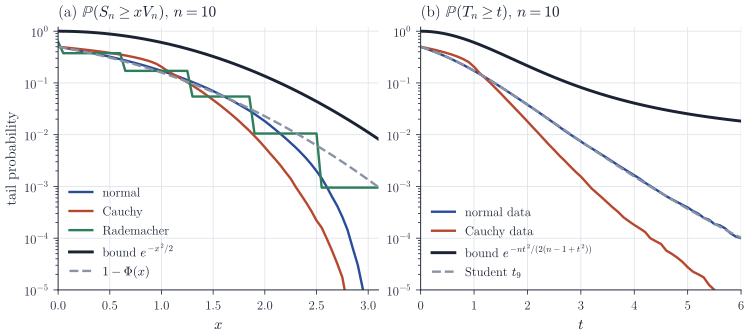
The bound is conservative. For \(n = 10\) and a one-sided level of \(0.05\), (2) requires \(t \ge 3.67\), against the Student quantile \(1.83\); as \(n \to \infty\) the threshold decreases to \(\sqrt{2\log 20} \approx 2.45\), against \(1.645\). What is bought with this conservatism is validity for every symmetric distribution at every sample size, including distributions without a mean.
Beyond symmetry
Symmetry cannot simply be dropped. Let \(X\) take the value \(-1\) with probability \(1 - p\) and \((1 - p)/p\) with probability \(p\), so that \(\E X = 0\). With probability \((1 - p)^n\) every observation equals \(-1\), and then \(W_n = -\sqrt n\). For \(n = 10\) and \(p = 0.001\) this event has probability \(0.990\), while \(e^{-n/2} \approx 0.0067\). No bound of the form \(\P(W_n \le -x) \le e^{-c x^2}\) can hold uniformly over mean-zero distributions: a rare large positive value is what keeps the mean at zero, and in a small sample it is usually absent. Without symmetry, a bound that holds for every mean-zero distribution needs a normalizer that contains more than the observed squares.
The canonical assumption
De la Peña, Klass and Lai (2004) organized the theory around the following condition, building on exponential inequalities for martingales and ratios in de la Peña (1999). A pair of random variables \((A, B)\) with \(B \ge 0\) satisfies the canonical assumption if
\[\E \exp\bigl(\lambda A - \lambda^2 B^2/2\bigr) \le 1 \qquad \text{for all } \lambda \in \R. \tag{3}\]In the sequential version, \((A_t, B_t)_{t \ge 0}\) is adapted to a filtration \((\mathcal F_t)\), \(A_0 = B_0 = 0\), and for each \(\lambda\) the process \(M^\lambda_t = \exp(\lambda A_t - \lambda^2 B_t^2/2)\) is a supermartingale. The quantity \(A\) plays the role of a sum, and \(B^2\) that of its quadratic variation.
Proposition 2. Let \(d_1, d_2, \dots\) be adapted to \((\mathcal F_t)\) and \(A_t = \sum_{s \le t} d_s\). The sequential canonical assumption holds in each of the following cases.
- The conditional law of \(d_t\) given \(\mathcal F_{t-1}\) is symmetric, and \(B_t^2 = \sum_{s \le t} d_s^2\).
- \(\E[d_t \mid \mathcal F_{t-1}] = 0\) and \(\E d_t^2 < \infty\), and \(B_t^2 = \sum_{s \le t} \bigl(d_s^2 + \E[d_s^2 \mid \mathcal F_{s-1}]\bigr)\).
- \(d_t = x_t \eta_t\), where \(x_t\) is \(\mathcal F_{t-1}\)-measurable, \(\eta_t\) is \(\mathcal F_t\)-measurable and conditionally \(\sigma\)-sub-Gaussian: almost surely, \(\int e^{\lambda u}\,Q_t(\dd u) \le e^{\lambda^2\sigma^2/2}\) for all \(\lambda \in \R\), where \(Q_t\) is a regular conditional distribution of \(\eta_t\) given \(\mathcal F_{t-1}\); and \(B_t^2 = \sigma^2 \sum_{s \le t} x_s^2\).
Proof. In each case \(M^\lambda_t = M^\lambda_{t-1} \exp(\lambda d_t - \lambda^2 (B_t^2 - B_{t-1}^2)/2)\), and it suffices to show that the conditional expectation of the last factor given \(\mathcal F_{t-1}\) is at most one.
(1) Averaging over the sign of \(d_t\), which is allowed by conditional symmetry, \(\E[e^{\lambda d_t - \lambda^2 d_t^2/2} \mid \mathcal F_{t-1}] = \E[\cosh(\lambda d_t) e^{-\lambda^2 d_t^2/2} \mid \mathcal F_{t-1}] \le 1\) because \(\cosh y \le e^{y^2/2}\).
(2) We first show \(e^{y - y^2/2} \le 1 + y + y^2/2\) for all real \(y\). The right side is \(((1+y)^2 + 1)/2 > 0\); let \(h(y) = \log(1 + y + y^2/2) - y + y^2/2\). Then \(h(0) = 0\) and
\[h'(y) = \frac{1 + y}{1 + y + y^2/2} - 1 + y = \frac{y\,(1 + y/2 + y^2/2)}{1 + y + y^2/2},\]whose sign is that of \(y\), because \(1 + y/2 + y^2/2 > 0\) (its discriminant is negative). So \(h \ge 0\). Applying the inequality with \(y = \lambda d_t\) and taking conditional expectations, with \(\sigma_t^2 = \E[d_t^2 \mid \mathcal F_{t-1}]\),
\[\E\bigl[e^{\lambda d_t - \lambda^2 d_t^2/2} \bigm\vert \mathcal F_{t-1}\bigr] \le 1 + \lambda^2 \sigma_t^2/2 \le e^{\lambda^2\sigma_t^2/2},\]and multiplying by the \(\mathcal F_{t-1}\)-measurable factor \(e^{-\lambda^2\sigma_t^2/2}\) gives the claim.
(3) Because \(x_t\) is \(\mathcal F_{t-1}\)-measurable, \(\E[e^{\lambda x_t \eta_t} \mid \mathcal F_{t-1}] = \int e^{\lambda x_t u}\,Q_t(\dd u)\) almost surely, and the bound, which holds for all real arguments simultaneously, can be evaluated at the random argument \(\lambda x_t\). This gives \(\E[e^{\lambda x_t\eta_t} \mid \mathcal F_{t-1}] \le e^{\lambda^2 x_t^2\sigma^2/2}\).
Case (2) is due to Bercu and Touati (2008); it needs only a finite variance, but the normalizer contains the predictable variance \(\sum_s \E[d_s^2 \mid \mathcal F_{s-1}]\), which is how the counterexample above is excluded. Case (3) is the form used in regression and bandit problems, where the normalizer is the design rather than the noise. Continuous-time analogues hold as well: for a continuous local martingale \(M\) with \(M_0 = 0\), \(\exp(\lambda M_t - \lambda^2 \langle M \rangle_t/2)\) is a nonnegative local martingale, hence a supermartingale, so \((M_t, \langle M\rangle_t^{1/2})\) satisfies the canonical assumption.
From the canonical assumption to a tail bound: the method of mixtures
Assumption (3) controls \(\exp(\lambda A - \lambda^2 B^2/2)\) for each fixed \(\lambda\). The value of \(\lambda\) that would turn it into a bound on \(A/B\) is \(\lambda = A/B^2\), where the exponent becomes \(A^2/(2B^2)\); but this value is random, and (3) says nothing about \(\E \sup_\lambda \exp(\lambda A - \lambda^2 B^2/2)\). The remedy, called pseudo-maximization in the survey of de la Peña, Klass and Lai (2007), is to integrate over \(\lambda\) instead of maximizing. An integral of the functions in (3) against a probability measure on \(\lambda\) still has expectation at most one, and with a Gaussian measure the integral is close to the maximum. The idea goes back to Robbins (1970).
Theorem 3 (normal mixture). Let \((A, B)\) satisfy (3) and let \(y > 0\), \(\delta \in (0, 1)\). Then
\[\P\Bigl(\abs{A} \ge \sqrt{(B^2 + y)\bigl(\log(1 + B^2/y) + 2\log(1/\delta)\bigr)}\Bigr) \le \delta.\]If \((A_t, B_t)_{t \ge 0}\) satisfies the sequential canonical assumption, then
\[\P\Bigl(\exists\, t \ge 0 : \abs{A_t} \ge \sqrt{(B_t^2 + y)\bigl(\log(1 + B_t^2/y) + 2\log(1/\delta)\bigr)}\Bigr) \le \delta.\]Proof. Let \(\gamma_y\) be the \(N(0, 1/y)\) density. Completing the square,
\[\bar M := \int_{\R} e^{\lambda A - \lambda^2 B^2/2}\, \gamma_y(\lambda)\, \dd\lambda = \sqrt{\frac{y}{2\pi}} \int_{\R} e^{\lambda A - \lambda^2 (B^2 + y)/2}\, \dd\lambda = \sqrt{\frac{y}{B^2 + y}}\, \exp\Bigl(\frac{A^2}{2(B^2 + y)}\Bigr).\]The integrand is nonnegative, so Tonelli’s theorem and (3) give \(\E \bar M = \int \E e^{\lambda A - \lambda^2B^2/2} \gamma_y(\lambda)\,\dd\lambda \le 1\), and Markov’s inequality gives \(\P(\bar M \ge 1/\delta) \le \delta\). Taking logarithms, \(\bar M \ge 1/\delta\) is exactly the event in the first display.
In the sequential case define \(\bar M_t\) in the same way from \((A_t, B_t)\). For each \(t\), conditional Tonelli and the supermartingale property of each \(M^\lambda\) give \(\E[\bar M_t \mid \mathcal F_{t-1}] = \int \E[M^\lambda_t \mid \mathcal F_{t-1}] \gamma_y(\lambda)\,\dd\lambda \le \bar M_{t-1}\), so \(\bar M\) is a nonnegative supermartingale with \(\bar M_0 = 1\). Ville’s inequality states that such a process satisfies \(\P(\bar M_t \ge 1/\delta \text{ for some } t) \le \delta\). To prove it, let \(\tau = \inf\{t : \bar M_t \ge 1/\delta\}\). For each \(m\), optional stopping at the bounded time \(\tau \wedge m\) gives \(\E \bar M_{\tau \wedge m} \le \E \bar M_0 = 1\), while \(\bar M_{\tau\wedge m} \ge 1/\delta\) on \(\{\tau \le m\}\); hence \(\P(\tau \le m) \le \delta\), and letting \(m \to \infty\) gives \(\P(\tau < \infty) \le \delta\).
Three features of the result deserve comment. First, the boundary is linear in \(B\) up to a logarithm, so \(A/B\) is controlled at the scale of a standard normal variable, with no constant supplied by the user. The free parameter \(y\) sets the scale at which the boundary is tightest relative to \(B\): for \(\delta = 0.05\) the ratio of the boundary to \(B\) is smallest, about \(3.04\), when \(B^2 \approx 8.2\,y\). Second, the time-uniform statement costs essentially nothing over the fixed-time one: the same inequality holds simultaneously for all \(t\), which is what makes it suitable for sequential monitoring and adaptive data collection. Third, the boundary grows like \(\sqrt{B_t^2 \log B_t^2}\), while the law of the iterated logarithm shows that no time-uniform boundary can be smaller than \(\sqrt{2 B_t^2 \log\log B_t^2}\) in order. The normal mixture overpays by replacing \(\log\log\) with \(\log\). Discrete mixtures and stitched boundaries recover the iterated-logarithm rate (Howard, Ramdas, McAuliffe and Sekhon, 2021). Fixed-sample versions of Theorem 3, in which \(y\) is replaced by a quantity such as \((\E B)^2\), together with moment bounds and laws of the iterated logarithm, are in de la Peña, Klass and Lai (2004).
How this differs from other concentration inequalities
The table summarizes the comparison for a sum of \(n\) independent or martingale-difference terms.
| Inequality | Event controlled | Where the scale comes from | Tail assumption | Holds uniformly in time |
|---|---|---|---|---|
| Hoeffding | \(S_n \ge t\) | ranges, known in advance | bounded summands | with a mixture or stitching argument |
| Bernstein, sub-Gaussian | \(S_n \ge t\) | variance or Orlicz norm, known in advance | bounded or sub-Gaussian | with a mixture or stitching argument |
| Freedman | \(S_n \ge t\) and \(\langle S\rangle_n \le v\) | bound \(v\) on the predictable variance | increments bounded above | yes, on \(\{\langle S\rangle_n \le v\}\) |
| Empirical Bernstein | \(\mu - \bar X_n \ge\) data-dependent level | sample variance, controlled separately | bounded, i.i.d. | separate versions exist |
| Self-normalized, symmetric (Theorem 1) | \(S_n \ge x V_n\) | observed \(V_n^2 = \sum_i X_i^2\) | none; symmetry | with the growing boundary of Theorem 3 |
| Self-normalized, canonical (Theorem 3) | \(\abs{A} \ge x\) times a function of \(B\) | observed or predictable \(B^2\) | the canonical assumption | yes |
Four differences stand out.
Deterministic versus random normalization. A classical bound controls \(\P(S_n \ge t)\); a self-normalized bound controls \(\P(S_n \ge x V_n)\). The second concerns a scale-free ratio, and under symmetry its bound does not depend on the distribution at all, even though the law of \(S_n/V_n\) does. Converting the first into a confidence interval requires plugging in an estimate of the scale and then controlling the error of that estimate, which is what the second-order term of the empirical Bernstein bound pays for.
Moments. Exponential bounds for \(S_n\) require exponential moments, or bounded summands, because the event \(\{S_n \ge t\}\) is genuinely affected by heavy tails. The event \(\{S_n \ge x V_n\}\) is not: a large observation inflates the normalizer as much as the sum. Theorem 1 holds for Cauchy data; Shao’s large deviation theorem holds without moments.
Dependence and adaptivity. Through the canonical assumption, the results apply to martingales, so the summands may be chosen adaptively, as in sequential experiments, bandits and stochastic regression. Freedman’s inequality is also a martingale inequality, but it controls \(S_n\) only on the event that the predictable variance stays below a level \(v\) fixed in advance. Self-normalized bounds let the threshold move with the realized quadratic variation: the observed squares under conditional symmetry, observed plus predictable variance in general.
What has to be paid. Without symmetry, bounds that hold for every distribution in a class need a normalizer with a predictable component (Proposition 2(2)) or a sub-Gaussian constant (Proposition 2(3)). The bounds have the Gaussian exponent but not the Gaussian constant, since \(e^{-x^2/2}\) exceeds \(1 - \Phi(x)\) by a factor of order \(x\), and the mixture bounds add logarithmic terms. Finally, nothing in this list covers ratios of the second kind, statistics divided by a power of their total; for these the relevant results are exact moment formulas, discussed at the end.
The mixture step is also the starting point of PAC-Bayesian bounds, which average an exponential supermartingale over a prior distribution on a parameter and then apply Markov’s or Ville’s inequality; in Theorem 3 the parameter is one-dimensional and the prior Gaussian.
Applications
Student’s t without normality
Theorem 1 gives a one-sided test of the hypothesis that the observations are independent and symmetric about \(\mu_0\), with no further assumption. Compute \(W_n\) from \(X_i - \mu_0\) and reject in favour of a larger centre when \(W_n \ge \sqrt{2\log(1/\delta)}\); the probability of rejection under the hypothesis is at most \(\delta\). By (1), when \(s_n > 0\) this is the same as \(T_n \ge t_\delta\) with \(t_\delta^2 = 2(n-1)\log(1/\delta)/(n - 2\log(1/\delta))\), which is the inversion of (2). Since \(\abs{W_n} \le \sqrt n\), the test can reject only when \(n > 2\log(1/\delta)\), that is \(n \ge 6\) for \(\delta = 0.05\). A two-sided test uses \(\delta/2\) in each tail. Under normality the test is less powerful than the \(t\)-test, as Figure 1(b) shows, but its level is guaranteed for heavy-tailed and discrete symmetric distributions at every sample size. Efron (1969) studied the behaviour of the usual \(t\)-test under symmetry in detail.
Anytime-valid inference
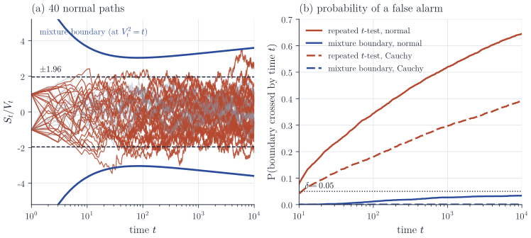
Suppose observations arrive one at a time and the analyst may stop whenever the evidence looks convincing. Repeating a fixed-sample test at every time point inflates its error probability: for data with finite variance and a two-sided test at nominal level \(0.05\), the probability that the statistic ever crosses \(\pm 1.96\) tends to one, by the law of the iterated logarithm. Figure 2 shows this for normal and Cauchy data. The time-uniform part of Theorem 3, applied with \(A_t = S_t\) and \(B_t^2 = V_t^2\) for symmetric observations (Proposition 2(1)), gives a boundary that the self-normalized sum crosses with probability at most \(\delta\) over the entire infinite horizon. Inverting it, the set
\[C_t = \Bigl\{\mu : \Bigl\lvert\sum_{s \le t}(X_s - \mu)\Bigr\rvert < \sqrt{\bigl(V_t^2(\mu) + y\bigr)\bigl(\log(1 + V_t^2(\mu)/y) + 2\log(1/\delta)\bigr)}\Bigr\},\]where \(V_t^2(\mu) = \sum_{s \le t}(X_s - \mu)^2\), contains the centre of symmetry \(\mu\) at every time \(t\) simultaneously with probability at least \(1 - \delta\), whatever the tails of the distribution. Such confidence sequences can be monitored continuously and stopped at any data-dependent time. Howard, Ramdas, McAuliffe and Sekhon (2021) develop this theory systematically, and Waudby-Smith and Ramdas (2024) construct confidence sequences for bounded observations by betting, which adapt to the unknown variance.
Least squares with adaptively chosen regressors
In stochastic regression the regressors are chosen by the experimenter, or by an algorithm, on the basis of past responses. The classical distribution theory for least squares treats the design as fixed and need not apply; Lai and Wei (1982) obtained strong consistency in this setting with martingale methods. The vector form of Theorem 3 gives a confidence set valid uniformly in time.
Theorem 4. Let \(x_t \in \R^d\) be \(\mathcal F_{t-1}\)-measurable and \(\eta_t\) be \(\mathcal F_t\)-measurable and conditionally \(\sigma\)-sub-Gaussian in the sense of Proposition 2(3). Let \(S_t = \sum_{s \le t} x_s\eta_s\), \(V_t = \sum_{s \le t} x_s x_s^\top\), and let \(\Lambda\) be a positive definite matrix. Then for \(\delta \in (0,1)\),
\[\P\Bigl(\exists\, t \ge 0: S_t^\top (V_t + \Lambda)^{-1} S_t \ge 2\sigma^2 \log\Bigl(\frac{\det(V_t + \Lambda)^{1/2}}{\delta\, \det(\Lambda)^{1/2}}\Bigr)\Bigr) \le \delta .\]Proof. For each \(\theta \in \R^d\), Proposition 2(3) applied to \(d_t = (\theta^\top x_t)\eta_t\) shows that \(M^\theta_t = \exp(\theta^\top S_t - \sigma^2\theta^\top V_t\theta/2)\) is a nonnegative supermartingale with \(M^\theta_0 = 1\). Mix over \(\theta \sim N(0, (\sigma^2\Lambda)^{-1})\). The Gaussian integral gives
\[\bar M_t = \Bigl(\frac{\det \Lambda}{\det(V_t + \Lambda)}\Bigr)^{1/2} \exp\Bigl(\frac{S_t^\top (V_t + \Lambda)^{-1} S_t}{2\sigma^2}\Bigr),\]which is a nonnegative supermartingale with \(\bar M_0 = 1\) by conditional Tonelli, exactly as in Theorem 3. Ville’s inequality and a rearrangement of \(\{\bar M_t \ge 1/\delta\}\) finish the proof.
For the model \(y_t = x_t^\top\theta^* + \eta_t\), the ridge estimator with penalty \(\kappa > 0\), \(\hat\theta_t = (V_t + \kappa I)^{-1}\sum_{s\le t} x_s y_s\), satisfies \(\hat\theta_t - \theta^* = (V_t + \kappa I)^{-1}(S_t - \kappa\theta^*)\). With \(\Lambda = \kappa I\) and \(\norm{v}_M = (v^\top M v)^{1/2}\), the triangle inequality and \((V_t + \kappa I)^{-1} \preceq \kappa^{-1} I\) give, with probability at least \(1-\delta\), for all \(t\) simultaneously,
\[\norm{\hat\theta_t - \theta^*}_{V_t + \kappa I} \le \sigma\sqrt{2\log\Bigl(\frac{\det(V_t + \kappa I)^{1/2}}{\delta\,\kappa^{d/2}}\Bigr)} + \sqrt\kappa\, \norm{\theta^*}_2 .\]This is the confidence ellipsoid of Abbasi-Yadkori, Pál and Szepesvári (2011), on which optimistic algorithms for linear bandits are built. The normalizer is the design matrix \(V_t\), which the data determine; the user supplies only the noise level \(\sigma\) and, to use the set, a bound on \(\norm{\theta^*}_2\).
Ratios normalized by a total
The second kind of self-normalization divides a statistic by a power of the sample total. Let \(X_1, \dots, X_n\) be i.i.d. nonnegative with distribution \(F\), Laplace transform \(L(\lambda) = \E e^{-\lambda X_1}\) and exponentially tilted law \(dF^{(\lambda)}(x) = e^{-\lambda x}\,dF(x)/L(\lambda)\). Two examples are the sample Gini coefficient and the sample squared coefficient of variation,
\[\widehat G = \frac{\sum_{i \ne j}\abs{X_i - X_j}}{2(n-1) S_n}, \qquad \widehat c_V^{\,2} = \frac{n}{n-1}\cdot\frac{\sum_{i<j}(X_i - X_j)^2}{S_n^2},\]which estimate \(G = \E\abs{X_1 - X_2}/(2\E X_1)\) and \(c_V^2 = \Var X_1/(\E X_1)^2\). Both are ratios \(U(X)/S_n^\beta\), with \(\beta = 1\) and \(\beta = 2\), \(U \ge 0\) and \(U(0) = 0\); on the event \(\{S_n = 0\}\), where all observations vanish, a value \(r\) is assigned by convention. Their bias does not follow from concentration inequalities, but it can be computed exactly.
Proposition 5 (Zou, Yao and de la Peña, 2025, Theorem 1 and Corollary 1). Let \(\beta > 0\), let \(U : [0,\infty)^n \to [0, \infty)\) be measurable with \(U(0) = 0\), and let \(Z = U(X)/S_n^\beta\) on \(\{S_n > 0\}\) and \(Z = r\) on \(\{S_n = 0\}\). Then
\[\E Z = \frac{1}{\Gamma(\beta)}\int_0^\infty \lambda^{\beta-1} L(\lambda)^n\, \E_{F^{(\lambda)}} U(X)\, \dd\lambda + r\, \P(X_1 = 0)^n,\]where \(\E_{F^{(\lambda)}}\) denotes expectation for i.i.d. observations from \(F^{(\lambda)}\). Both sides may be infinite; the paper states the result for \(U\) with finite expectation and also allows non-identically distributed observations.
Proof. For \(s > 0\), \(s^{-\beta} = \Gamma(\beta)^{-1}\int_0^\infty \lambda^{\beta-1}e^{-\lambda s}\,\dd\lambda\). Hence on \(\{S_n > 0\}\), \(Z = \Gamma(\beta)^{-1}\int_0^\infty \lambda^{\beta-1}\,U(X)\,e^{-\lambda S_n}\,\dd\lambda\), and on \(\{S_n = 0\}\) the same integral vanishes because \(U(0) = 0\). The integrand is nonnegative, so by Tonelli’s theorem \(\E[Z; S_n > 0] = \Gamma(\beta)^{-1}\int_0^\infty \lambda^{\beta-1}\,\E[U(X) e^{-\lambda S_n}]\,\dd\lambda\). Finally, \(e^{-\lambda S_n}\prod_i dF(x_i) = L(\lambda)^n \prod_i dF^{(\lambda)}(x_i)\), so \(\E[U(X)e^{-\lambda S_n}] = L(\lambda)^n\,\E_{F^{(\lambda)}}U(X)\); and \(\{S_n = 0\} = \{X_1 = \dots = X_n = 0\}\) has probability \(\P(X_1 = 0)^n\).
The device is the same as in the method of mixtures: a nonlinear function of the sum, here \(S_n^{-\beta}\) and there \(\exp(A^2/(2(B^2+y)))\), is written as an integral of exponentials of the sum, and exponentials of sums factorize over independent observations. When \(U\) is a \(U\)-statistic of fixed order, \(\E_{F^{(\lambda)}}U\) involves only a fixed number of observations, so the cost of evaluating the formula does not grow with \(n\).
For the Gini coefficient, \(\beta = 1\) and \(U = \sum_{i \ne j}\abs{X_i - X_j}/(2(n-1))\), and the formula becomes
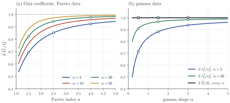
\[\E\widehat G = \frac n2 \int_0^\infty \E\bigl[\abs{X_1 - X_2}\,e^{-\lambda(X_1 + X_2)}\bigr]\, L(\lambda)^{n-2}\,\dd\lambda + r\,\P(X_1 = 0)^n .\]Two cases can be done by hand. For gamma data, \(X_i \sim \mathrm{Gamma}(\alpha, 1)\), the total \(S_n\) is independent of the vector \((X_1, \dots, X_n)/S_n\), which has a Dirichlet distribution; this is classical, and Lukacs (1955) proved the converse, that independence of \(X_1 + X_2\) and \(X_1/(X_1 + X_2)\) characterizes the gamma family. Since \(\widehat G\) and \(\widehat c_V^{\,2}\) are functions of that vector, \(\E U = \E[\widehat G\, S_n] = \E\widehat G\,\E S_n\) and similarly for \(\widehat c_V^{\,2}\). This gives \(\E\widehat G = G\) for every \(n\), a fact first proved by Baydil, de la Peña, Zou and Yao (2025), and
\[\E\,\widehat c_V^{\,2} = \frac{n}{n-1}\cdot\frac{\E\sum_{i<j}(X_i - X_j)^2}{\E S_n^2} = \frac{n}{n-1}\cdot\frac{n(n-1)\alpha}{n\alpha + n^2\alpha^2} = \frac{n}{n\alpha + 1},\]so that \(\E\,\widehat c_V^{\,2}/c_V^2 = n\alpha/(n\alpha + 1) < 1\). Proposition 5 gives the same values: the tilted law is \(\mathrm{Gamma}(\alpha, 1 + \lambda)\), \(L(\lambda) = (1+\lambda)^{-\alpha}\), and the integrals are beta integrals. For Pareto data, \(\P(X > x) = x^{-\alpha}\) on \([1, \infty)\) with \(\alpha > 1\) and \(G = 1/(2\alpha - 1)\), no closed form is available, but the formula reduces the expectation to a low-dimensional integral that can be evaluated numerically for any \(n\). Figure 3 shows the result: the sample Gini coefficient underestimates inequality, by about 31% for \(n = 5\) and \(\alpha = 1.5\) and still by about 9% for \(n = 20\) and \(\alpha = 2\). The heavier the tail, the larger the bias, because the largest observations, which carry most of the inequality, are the ones a small sample misses. Zou, Yao and de la Peña (2025) use such formulas to construct bias corrections, by evaluating the bias at a fitted parameter value and subtracting it; the correction is only as good as the parametric model used to compute it.
Further reading
The survey of de la Peña, Klass and Lai (2007) is the shortest route into the exponential inequalities, and the monograph of de la Peña, Lai and Shao (2009) covers both the inequalities and the limit theory, including Studentized \(U\)-statistics and self-normalized laws of the iterated logarithm. Howard, Ramdas, McAuliffe and Sekhon (2020) give a unified treatment of time-uniform bounds through nonnegative supermartingales, in which many classical inequalities, including Freedman’s and those under the canonical assumption, arise from a single construction.
References
- Y. Abbasi-Yadkori, D. Pál and Cs. Szepesvári, “Improved algorithms for linear stochastic bandits”, Advances in Neural Information Processing Systems 24, 2011.
- B. Baydil, V. H. de la Peña, H. Zou and H. Yao, “Unbiased estimation of the Gini coefficient”, Statistics and Probability Letters, 2025.
- B. Bercu and A. Touati, “Exponential inequalities for self-normalized martingales with applications”, Annals of Applied Probability 18 (2008), 1848–1869.
- S. Boucheron, G. Lugosi and P. Massart, Concentration Inequalities: A Nonasymptotic Theory of Independence, Oxford University Press, 2013.
- V. H. de la Peña, “A general class of exponential inequalities for martingales and ratios”, Annals of Probability 27 (1999), 537–564.
- V. H. de la Peña, M. J. Klass and T. L. Lai, “Self-normalized processes: exponential inequalities, moment bounds and iterated logarithm laws”, Annals of Probability 32 (2004), 1902–1933.
- V. H. de la Peña, M. J. Klass and T. L. Lai, “Pseudo-maximization and self-normalized processes”, Probability Surveys 4 (2007), 172–192.
- V. H. de la Peña, T. L. Lai and Q.-M. Shao, Self-Normalized Processes: Limit Theory and Statistical Applications, Springer, 2009.
- G. P. Chistyakov and F. Götze, “Limit distributions of Studentized means”, Annals of Probability 32 (2004), 28–77.
- B. Efron, “Student’s t-test under symmetry conditions”, Journal of the American Statistical Association 64 (1969), 1278–1302.
- D. A. Freedman, “On tail probabilities for martingales”, Annals of Probability 3 (1975), 100–118.
- E. Giné, F. Götze and D. M. Mason, “When is the Student t-statistic asymptotically standard normal?”, Annals of Probability 25 (1997), 1514–1531.
- S. R. Howard, A. Ramdas, J. McAuliffe and J. Sekhon, “Time-uniform Chernoff bounds via nonnegative supermartingales”, Probability Surveys 17 (2020), 257–317.
- S. R. Howard, A. Ramdas, J. McAuliffe and J. Sekhon, “Time-uniform, nonparametric, nonasymptotic confidence sequences”, Annals of Statistics 49 (2021), 1055–1080.
- B.-Y. Jing, Q.-M. Shao and Q. Wang, “Self-normalized Cramér-type large deviations for independent random variables”, Annals of Probability 31 (2003), 2167–2215.
- T. L. Lai and C. Z. Wei, “Least squares estimates in stochastic regression models with applications to identification and control of dynamic systems”, Annals of Statistics 10 (1982), 154–166.
- B. F. Logan, C. L. Mallows, S. O. Rice and L. A. Shepp, “Limit distributions of self-normalized sums”, Annals of Probability 1 (1973), 788–809.
- E. Lukacs, “A characterization of the gamma distribution”, Annals of Mathematical Statistics 26 (1955), 319–324.
- A. Maurer and M. Pontil, “Empirical Bernstein bounds and sample variance penalization”, Conference on Learning Theory (COLT), 2009.
- H. Robbins, “Statistical methods related to the law of the iterated logarithm”, Annals of Mathematical Statistics 41 (1970), 1397–1409.
- Q.-M. Shao, “Self-normalized large deviations”, Annals of Probability 25 (1997), 285–328.
- Q.-M. Shao, “A Cramér type large deviation result for Student’s t-statistic”, Journal of Theoretical Probability 12 (1999), 385–398.
- J. Ville, Étude critique de la notion de collectif, Gauthier-Villars, 1939.
- I. Waudby-Smith and A. Ramdas, “Estimating means of bounded random variables by betting”, Journal of the Royal Statistical Society Series B 86 (2024), 1–27.
- H. Zou, H. Yao and V. H. de la Peña, “A scalable formula for the moments of a family of self-normalized statistics”, arXiv:2509.14428, 2025.