Whitening transformations: a rotation’s worth of solutions and how to choose one

Whitening replaces a random vector $X$ by a linear transformation $Z = W(X - \mu)$ whose coordinates are uncorrelated with unit variance. It is a common preprocessing step, for instance before independent component analysis or before fitting models that assume isotropic inputs, and it is the population version of standardizing a data matrix in all directions at once. The constraint $\Cov(Z) = I$ does not determine $W$: any rotation of a whitened vector is still white. Below are the full set of solutions, the three choices in common use, and the optimality property that distinguishes each.

Throughout, $X$ is a random vector in $\R^p$ with mean $\mu$ and covariance $\Sigma \succ 0$, and $Y = X - \mu$. Write $\Sigma = U\Lambda U^\top$ with $U$ orthogonal, $\Lambda = \diag(\lambda_1, \dots, \lambda_p)$ and $\lambda_1 \ge \cdots \ge \lambda_p > 0$, and $\Sigma^{\pm 1/2} = U\Lambda^{\pm 1/2}U^\top$. No distributional assumption beyond finite second moments is used.

All whitening matrices

A matrix $W \in \R^{p \times p}$ is a whitening matrix for $\Sigma$ if $\Cov(WY) = W\Sigma W^\top = I_p$. Taking determinants shows that $W$ is invertible, and then $W\Sigma W^\top = I_p$ is equivalent to $W^\top W = \Sigma^{-1}$.

Proposition 1. $W$ is a whitening matrix for $\Sigma$ if and only if $W = Q\Sigma^{-1/2}$ for an orthogonal matrix $Q$, and then $Q = W\Sigma^{1/2}$.

Proof. If $W = Q\Sigma^{-1/2}$ then $W\Sigma W^\top = Q\Sigma^{-1/2}\Sigma\Sigma^{-1/2}Q^\top = QQ^\top = I_p$. Conversely, if $W\Sigma W^\top = I_p$, put $Q = W\Sigma^{1/2}$; then $QQ^\top = W\Sigma W^\top = I_p$ and $Q\Sigma^{-1/2} = W$.

So whitening is always “Mahalanobis whitening followed by a rotation or reflection”. The second step is invisible to second moments, and any criterion that selects a particular $W$ must look at something other than $\Cov(Z)$. A natural candidate is the cross-covariance between the whitened and the original variables,

\[\Phi = \Cov(Z, Y) = W\Sigma = Q\Sigma^{1/2},\]

which records how each $Z_i$ relates to each $Y_j$. Three standard choices are:

ZCA or Mahalanobis whitening, $W = \Sigma^{-1/2}$, that is $Q = I_p$;
PCA whitening, $W = \Lambda^{-1/2}U^\top$, which projects onto the principal axes and rescales, $Q = U^\top$;
Cholesky whitening, $W = L^{-1}$ where $\Sigma = LL^\top$ with $L$ lower triangular, $Q = L^{-1}\Sigma^{1/2}$.

Figure 1 shows what the rotation does. A uniform distribution on a parallelogram has, after any whitening, a uniform distribution on a square with identity covariance, and the three choices produce three differently oriented squares.

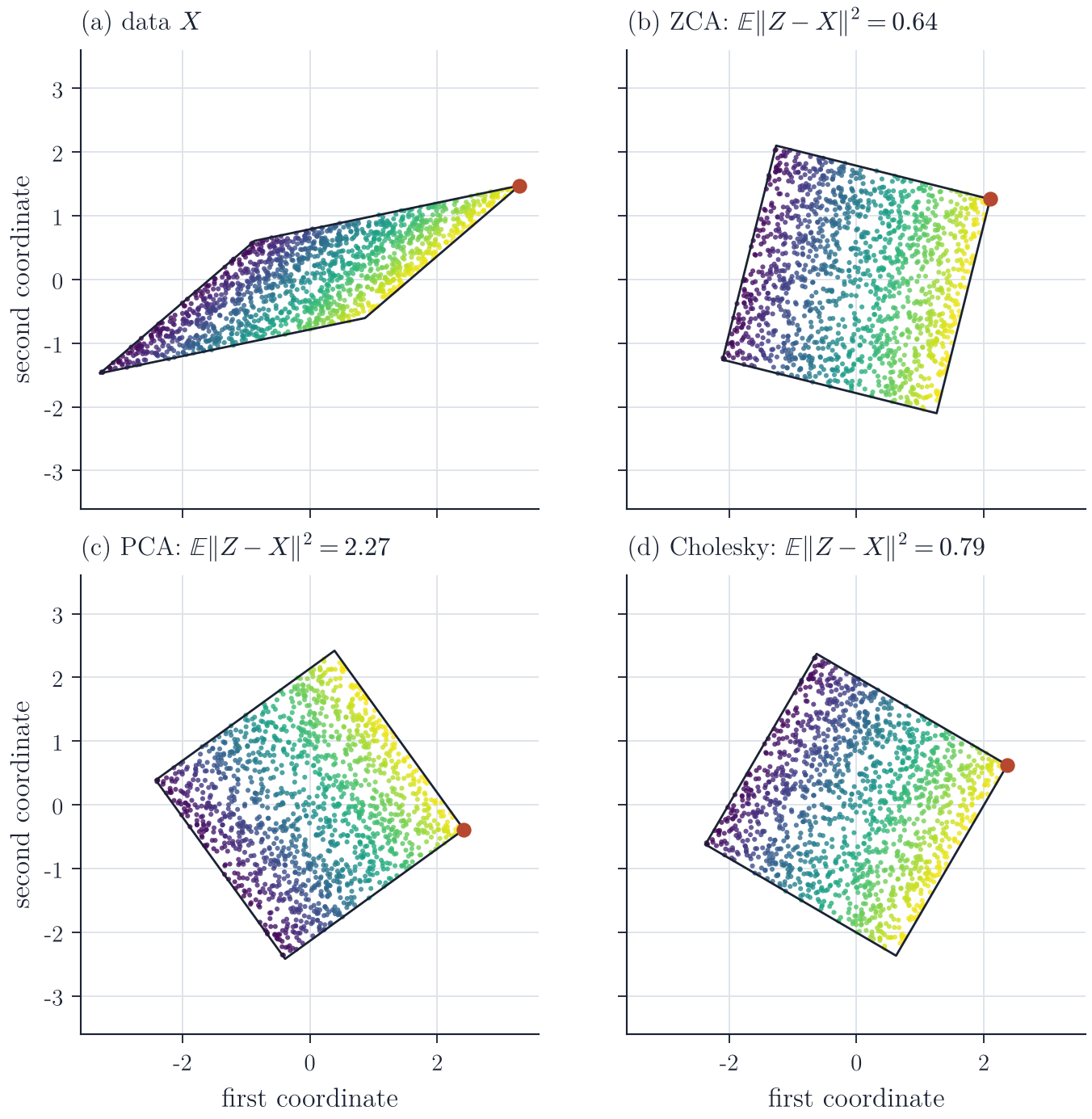
A uniform parallelogram and three whitened versions of it, each a square in a different orientation — Figure 1. (a) 1500 draws from a uniform distribution on a parallelogram, $X = MS$ with $S$ uniform on $[-\sqrt3, \sqrt3]^2$ and $M = \begin{pmatrix} 1.2 & 0.7 \\ 0.25 & 0.6\end{pmatrix}$, coloured by $S_1$; the red dot marks one corner. (b)–(d) The same draws after three whitening transformations. Each result is a square of side $2\sqrt3$, rotated or reflected differently. Panel titles give the population value of $\mathbb E\lVert Z - X\rVert^2$, which ZCA whitening minimizes.

ZCA whitening: the least change

Theorem 2. Among all whitening matrices for $\Sigma$, the mean squared distance $\E\lVert WY - Y\rVert^2$ is minimized uniquely by $W = \Sigma^{-1/2}$, with minimum value $\sum_{j}(1 - \sqrt{\lambda_j})^2$. Equivalently, $W = \Sigma^{-1/2}$ uniquely maximizes $\tr\Phi = \sum_j \Cov(Z_j, Y_j)$.

Proof. For any whitening matrix,

\[\E\lVert WY - Y\rVert^2 = \tr\bigl(\Cov(WY)\bigr) - 2\tr\bigl(\Cov(WY, Y)\bigr) + \tr(\Sigma) = p + \tr\Sigma - 2\tr(W\Sigma),\]

so the two criteria are equivalent. Write $W = Q\Sigma^{-1/2}$ by Proposition 1. Then $\tr(W\Sigma) = \tr(Q\Sigma^{1/2}) = \sum_j \sqrt{\lambda_j}\, u_j^\top Q u_j$, where $u_j$ are the columns of $U$. By the Cauchy–Schwarz inequality $u_j^\top Q u_j \le \lVert u_j\rVert\,\lVert Qu_j\rVert = 1$, with equality if and only if $Qu_j = u_j$. All $\lambda_j$ are positive, so the sum is at most $\sum_j \sqrt{\lambda_j}$, with equality if and only if $Q$ fixes every $u_j$, that is $Q = I_p$. Substituting $\tr(\Sigma^{-1/2}\Sigma) = \sum_j \sqrt{\lambda_j}$ gives the minimum value $\sum_j (1 - 2\sqrt{\lambda_j} + \lambda_j)$.

ZCA whitening therefore produces the white vector that stays closest to the original one, which is why it is preferred when the coordinates have a meaning that should survive whitening, such as pixel positions in an image: each $Z_j$ remains mostly a function of $Y_j$ and its correlated neighbours. It is also equivariant under rotations of the data. If $Y$ is replaced by $RY$ with $R$ orthogonal, the covariance becomes $R\Sigma R^\top$, whose inverse square root is $R\Sigma^{-1/2}R^\top$, and the whitened vector becomes $R\Sigma^{-1/2}R^\top RY = RZ$.

ZCA whitening is not invariant to rescaling individual coordinates, because the criterion $\E\lVert WY - Y\rVert^2$ adds squared errors in the original units. If the variables are measured on unrelated scales, the analogous criterion compares $Z$ with the standardized vector $V^{-1/2}Y$, where $V = \diag(\Sigma)$. Writing $P = V^{-1/2}\Sigma V^{-1/2}$ for the correlation matrix, every whitening matrix has the form $W = \tilde W V^{-1/2}$ with $\tilde W$ a whitening matrix for $P$, and Theorem 2 applied to $V^{-1/2}Y$ shows that

\[W = P^{-1/2}V^{-1/2}\]

uniquely minimizes $\E\lVert WY - V^{-1/2}Y\rVert^2$. Since $\Corr(Z_j, Y_j) = (W\Sigma V^{-1/2})_{jj} = (\tilde W P)_{jj}$, this choice, often called ZCA-cor, uniquely maximizes the sum of correlations $\sum_j \Corr(Z_j, Y_j)$.

PCA whitening: concentrating the information

PCA whitening ignores the original coordinates. Its whitened variables are the standardized principal components $Z_j = \lambda_j^{-1/2} u_j^\top Y$, and it is optimal for a different criterion: the rows of $\Phi$ are as unequal as possible. The squared norm of row $i$ of $\Phi = Q\Sigma^{1/2}$ is

\[\sum_{j=1}^p \Cov(Z_i, Y_j)^2 = q_i^\top \Sigma\, q_i ,\]

where $q_i^\top$ is the $i$th row of $Q$. These numbers sum to $\tr\Sigma$ for every whitening. For each $k$, the Ky Fan maximum principle (Horn and Johnson, Matrix Analysis) gives

\[\sum_{i=1}^k q_i^\top\Sigma q_i \le \lambda_1 + \cdots + \lambda_k\]

for any orthonormal $q_1, \dots, q_k$, with equality when $q_i = u_i$. PCA whitening attains the bound for every $k$ simultaneously: its first $k$ components carry the largest possible share of the total squared cross-covariance with $Y$. This is the property that makes it the right choice before discarding components, and the reason it is used for dimension reduction combined with whitening. The price is non-uniqueness: each $u_j$ is determined only up to sign, and only up to rotation within an eigenspace when eigenvalues repeat, so PCA-whitened data can change discontinuously under small perturbations of $\Sigma$. In Figure 1 the sign convention makes $U^\top$ a reflection, so the squares in panels (b) and (c) are mirror images of each other, and the distance to the original data is more than three times larger for PCA whitening.

Cholesky whitening: whitening in order

Because $L^{-1}$ is lower triangular, Cholesky whitening produces $Z_1$ from $Y_1$ alone, $Z_2$ from $(Y_1, Y_2)$, and so on. It is the only whitening matrix that is lower triangular with positive diagonal: if $W$ is such a matrix, $W^{-1}$ is lower triangular with positive diagonal and $W^{-1}W^{-\top} = \Sigma$, so $W^{-1} = L$ by uniqueness of the Cholesky factorization. Its components are standardized innovations,

\[Z_j = \frac{Y_j - \mathcal L(Y_j \mid Y_1, \dots, Y_{j-1})}{\sqrt{\Var\bigl(Y_j - \mathcal L(Y_j \mid Y_1, \dots, Y_{j-1})\bigr)}},\]

where $\mathcal L(\cdot \mid \cdot)$ denotes the best linear predictor; for Gaussian $X$ these are conditional expectations. To see this, note that $Y_{<j}$ and $Z_{<j}$ are invertible linear functions of each other, so they span the same space of linear combinations; $Z_j$ is uncorrelated with $Z_{<j}$, hence with $Y_{<j}$; and $Y_j = \sum_{i \le j} L_{ji}Z_i$ with $L_{jj} > 0$. Cholesky whitening is natural when the variables have an order, as in time series, where it computes the standardized one-step prediction errors of the series. Without a natural order it has no particular claim: permuting the variables changes the result.

Estimated covariances

In practice $\Sigma$ is replaced by a sample covariance $S$, and everything above applies to the empirical distribution with $S$ in place of $\Sigma$, provided $S \succ 0$, which requires at least $p + 1$ observations in general position. When $p$ is not small relative to $n$, the smallest eigenvalues of $S$ are biased downwards and $S^{-1/2}$ amplifies the directions they belong to, which are mostly noise. Common remedies are to add a small multiple of the identity before taking the inverse square root, to use a shrinkage estimator of $\Sigma$, or to discard the components with small eigenvalues, which is natural in PCA whitening.

Remarks

Whitening also clarifies what independent component analysis has to estimate. If $X = AS$ with $A$ invertible and independent, non-Gaussian, centred, unit-variance sources $S$, then any whitening gives $Z = WAS$ with $(WA)(WA)^\top = \Cov(Z) = I_p$, so $WA$ is orthogonal. After whitening only an orthogonal matrix remains unknown; second moments carry no information about it, and it is identified, up to permutation and signs of the sources, by non-Gaussianity. The comparison of whitening procedures through the cross-covariance and cross-correlation matrices, and the optimality results for ZCA, ZCA-cor and PCA whitening in this form, are due to Kessy, Lewin and Strimmer, “Optimal whitening and decorrelation” (The American Statistician, 2018), which also discusses the analogous PCA-cor variant.