Binh Ho
$\chi$ divergence upper bound (CUBO)
Minimizing the $\chi^2$ divergence between a true posterior and an approximate posterior is equivalent to minimizing an upper bound on the log marginal likelihood.
Introduction
Variational inference is typically performed by minimizing the reverse KL divergence between the true posterior and an approximate posterior. However, arbitrary divergences can also be used. In practice, choosing an appropriate divergence requires a balance of computational considerations and an assessment of the goal in mind. The reverse KL divergence is attractive because the resulting evidence lower bound (ELBO) is often easy to optimize.
An alternative to the reverse KL divergence for variational inference is the $\chi^2$ divergence. Originally proposed by Dieng et al., minimizing the $\chi^2$ divergence results in an upper bound on the log marginal likelihood. This provides a nice counterpart to the KL divergence’s resulting lower bound.
$\chi$ divergence and the CUBO
The $\chi^2$ divergence between $p$ and $q$ is given by
\[D_{\chi^2}(p(z | x) \| q(z)) = \mathbb{E}_{q(z)}\left[ \left(\frac{p(z | x)}{q(z)}\right)^2 - 1 \right].\]Expanding the posterior, we can pull out the evidence $p(x)$,
\begin{align} D_{\chi^2}(p(z | x) | q(z)) + 1 &= \mathbb{E}_{q(z)}\left[ \left(\frac{p(x, z)}{p(x) q(z)}\right)^2 \right] \\ &= \frac{1}{p(x)^2} \mathbb{E}_{q(z)}\left[ \left(\frac{p(x, z)}{q(z)}\right)^2 - 1 \right]. \\ \end{align}
Taking a log on both sides, we have
\[\log \left( D_{\chi^2}(p(z | x) \| q(z)) + 1\right) = -2 \log p(x) + \log \mathbb{E}_{q(z)}\left[ \left(\frac{p(x, z)}{q(z)}\right)^2 \right].\]Notice that the left hand side is nonnegative. To see this, note that $D_{\chi^2}\geq 0$ (because it’s a divergence), so $\log (D_{\chi^2} + 1) \geq \log(0+1) = 0$. Thus, rearranging terms again, we can obtain an upper bound on the log evidence,
\[\log p(x) \leq \mathcal{U} := \frac12 \log \mathbb{E}_{q(z)}\left[ \left(\frac{p(x, z)}{q(z)}\right)^2 \right].\]Here, $\mathcal{U}$ is known as the chi-divergence upper bound (CUBO), which was proposed by Dieng et al..
Minimizing the CUBO
Similar to the way that the ELBO is used in variational inference, we can optimize a variational approximation $q$ by minimizing the CUBO with respect to the variational parameters.
However, because the $\log$ appears outside the expectation in the CUBO, we cannot directly use a Monte Carlo approximation. Instead, consider the exponentiated CUBO,
\[\exp (2 \mathcal{U}) = \mathbb{E}_{q(z)}\left[ \left(\frac{p(x, z)}{q(z)}\right)^2 \right].\]We can approximate this quantity with Monte Carlo sampling. Specifically, we can estimate it with $T$ samples from $q$,
\[\exp (\mathcal{U}) \approx \frac1T \sum\limits_{t=1}^T \left(\frac{p(x, \widetilde{z}_t)}{q(\widetilde{z}_t)}\right)^2, ~~~ \widetilde{z}_t \sim q(z).\]Minimizing this quantity is equivalent to minimizing the CUBO due to the monotonicity of $\exp$ and $\log$. In practice, to evaluate this quantity we use take a log of the quantity inside the summation, and re-exponentiate it. In particular,
\[\frac1T \sum\limits_{t=1}^T \exp\left\{2\left(\log p(x, \widetilde{z}_t) - \log q(\widetilde{z}_t)\right)\right\}, ~~~ \widetilde{z}_t \sim q(z).\]Several methods have been proposed to reduce the variance of this estimator. One method is the reparameterization trick, as proposed by Dieng et al. Here, we write $z$ as the output of a deterministic function of the variational parameters $\lambda$ and an independent random variable $\epsilon$,
\[z = g(\lambda, \epsilon), ~~~ \epsilon \sim f.\]Using this trick, we can rewrite the Monte Carlo CUBO estimator as
\[L = \frac1T \sum\limits_{t=1}^T \left(\frac{p(x, g(\lambda, \epsilon_t))}{q(g(\lambda, \epsilon_t))}\right)^2, ~~~ \epsilon_t \sim f.\]To minimize the CUBO, we’ll use gradient-based methods. Let’s compute the gradient of $L$ with respect to $\lambda$. Using the chain rule, we have
\[\nabla_\lambda L = \frac2T \sum\limits_{t=1}^T \left(\frac{ p(x, g(\lambda, \epsilon_t))}{ q(g(\lambda, \epsilon_t))}\right) \nabla_\lambda \left[\frac{ p(x, g(\lambda, \epsilon_t))}{ q(g(\lambda, \epsilon_t))}\right]\]Expanding the gradient on the RHS,
\[\nabla_\lambda L = \frac2T \sum\limits_{t=1}^T \left(\frac{ p(x, g(\lambda, \epsilon_t))}{ q(g(\lambda, \epsilon_t))}\right) \nabla_\lambda \left[\exp\left\{ \log p(x, g(\lambda, \epsilon_t)) - \log q(g(\lambda, \epsilon_t))\right\}\right].\]Expanding the gradient once more and then collapsing terms, we have
\[\nabla_\lambda L = \frac2T \sum\limits_{t=1}^T \left(\frac{ p(x, g(\lambda, \epsilon_t))}{ q(g(\lambda, \epsilon_t))}\right)^2 \nabla_\lambda \left( \log \frac{p(x, g(\lambda, \epsilon_t))}{q(g(\lambda, \epsilon_t))} \right).\]We can use this gradient to minimize the CUBO and obtain a variational approximation $q$.
Mode-covering behavior of the $\chi^2$ divergence
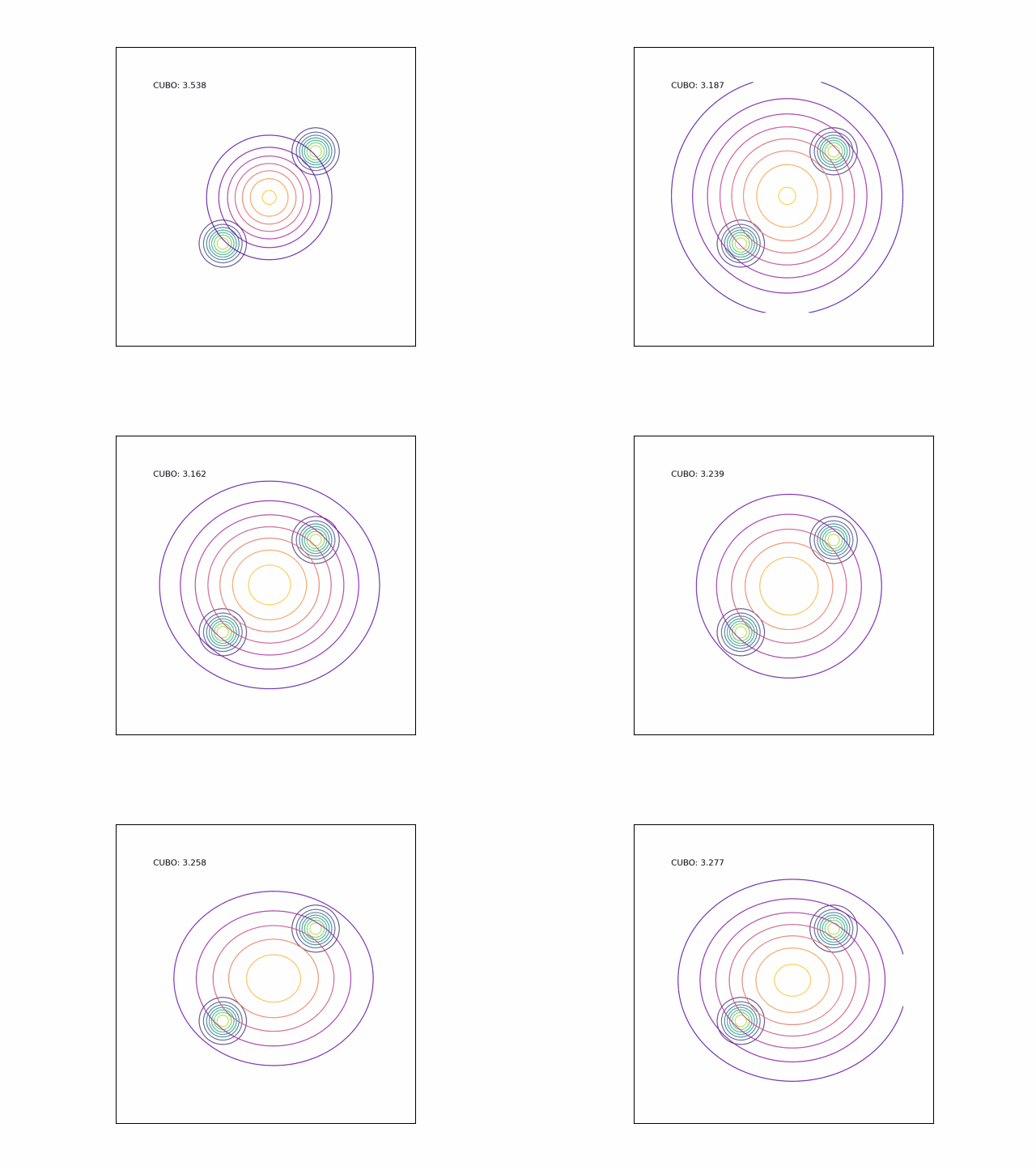
Recall that the KL divergence has mode seeking behavior. In other words, the KL divergence will be infinite whenever $p=0$ but $q>0$, so minima of the KL divergence tend to find “conservative” orientations of $q$ that just cover one mode of the true distribution $p$.
In contrast the $\chi^2$ divergence is “mode-covering”. In other words, it’s infinite whenever $p>0$ but $q=0$. This encourages solutions that tend to spread out the mass of $q$ as wide as possible to cover most of the mass of $p$. We will demonstrate this behavior in the experiments below.
Experiments
Unimodal Gaussian
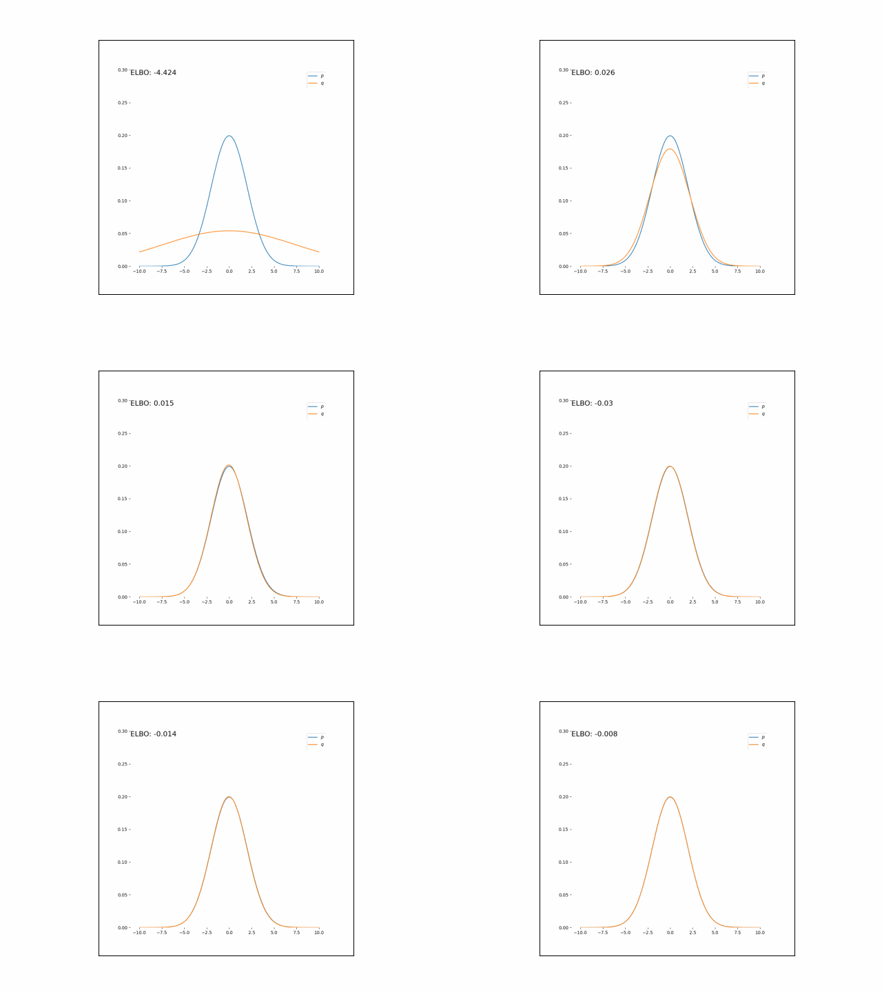
Consider a very simple experiment: approximating a one-dimensional Gaussian with another one-dimensional Gaussian. Specifically,
\begin{align} p(x) &= \mathcal{N}(0, 1) \\ q(x) &= \mathcal{N}(\lambda_\mu, \lambda_{\sigma^2}). \end{align}
Here, we’ll minimize the CUBO w.r.t. $\lambda_\mu$ an $\lambda_{\sigma^2}$. The animations below show the distributions over iterations of optimization (here, we use Adam to optimize the variational parameters).


As we can see, the CUBO spreads the mass of the variational Gaussian wider than the true Gaussian, resulting in an overestimate of the variance.
Bimodal Gaussian
We can see the difference in behavior between the CUBO and ELBO even more clearly in the case of a multimodal $p$. Below, we consider a two-dimensional Gaussian with two modes. We use a multivariate $t$-distribution as our approximate distribution.


Code
Code for the one-dimensional Gaussian experiment is below.
import matplotlib.pyplot as plt
from autograd import grad, value_and_grad, vector_jacobian_product
import autograd.numpy as np
from functools import partial
from autograd.scipy.stats import t, norm
from scipy.special import loggamma
from autograd.core import getval
from autograd.numpy import random as npr
from autograd.misc.optimizers import adam
from functools import partial
from scipy.special import logsumexp
import autograd.scipy.stats.t as t_dist
from viabel.optimization import RMSProp
from viabel.objectives import ExclusiveKL, AlphaDivergence
from scipy.stats import multivariate_normal as mvn
from autograd.scipy.stats import multivariate_normal

import matplotlib.animation as animation
import matplotlib.image as mpimg
import os

# use cubo if true, elbo if false
CUBO_FLAG = False
MULTIMODAL_FLAG = True


if MULTIMODAL_FLAG:
	class Model():

		def __init__(self, mean1, mean2, stddev1, stddev2):
			self.mean1 = mean1
			self.mean2 = mean2
			self.stddev1 = stddev1
			self.stddev2 = stddev2

		def log_density(self, zs):
			mode1_logdensity = np.log(0.5) + norm.logpdf(zs, self.mean1, self.stddev1)
			mode2_logdensity = np.log(0.5) + norm.logpdf(zs, self.mean2, self.stddev2)
			return np.logaddexp(mode1_logdensity, mode2_logdensity)

		# def sample(self, n):
		# 	num_clust1 = np.random.binomial(n=n, p=0.5)
		# 	num_clust2 = n - num_clust1
		# 	samples_mode1 = norm.rvs(self.mean1, self.stddev1, size=num_clust1)
		# 	samples_mode2 = norm.rvs(self.mean2, self.stddev2, size=num_clust2)
		# 	samples = np.concatenate([samples_mode1, samples_mode2])
		# 	return samples

else:

	class Model():

		def __init__(self, mean, stddev):
			self.mean = mean
			self.stddev = stddev

		def log_density(self, zs):
			return norm.logpdf(zs, self.mean, self.stddev)

		def sample(self, n):
			return norm.rvs(self.mean, self.stddev, size=n)


class ApproxMFGaussian():

	def __init__(self):
		pass

	def log_density(self, var_param, z):
		# variational density evaluated at samples
		return norm.logpdf(z, var_param[0], np.exp(var_param[1]))

	def sample(self, var_param, S):
		stddev = np.exp(var_param[1])
		return var_param[0] + seed.randn(S) * stddev

	# def entropy(self, var_param):
	# 	return 0.5 * (np.log(2*np.pi) + 1) + var_param[1] * 2

	def entropy(self, var_param):
		return 0.5 * 1 * (1.0 + np.log(2*np.pi)) + var_param[1] * 2

class ApproxMFT():
	"""A mean-field Student's t approximation family."""
	def __init__(self, df):
		self.df = df

	def log_density(self, var_param, x):
		return t_dist.logpdf(x, self.df, var_param[0], np.exp(var_param[1]))

	def sample(self, var_param, S):
		return var_param[0] + np.exp(var_param[1]) * seed.standard_t(self.df, size=S)


if __name__ == "__main__":

	n = 1000
	d = 1
	n_iter = 400

	# Generate data
	if MULTIMODAL_FLAG:
		model = Model(mean1=-6.0, mean2=6.0, stddev1=1.0, stddev2=1.0)
	else:
		mean = 0.0
		stddev = 1
		model = Model(mean=mean, stddev=stddev)
	approx = ApproxMFGaussian()
	# approx = ApproxMFT(df=2)

	S = 1000
	variational_mean = 0.0
	variational_log_stddev_diag = 0.0
	var_param = np.array([variational_mean, variational_log_stddev_diag])
	seed = npr.RandomState(0)

	def compute_log_weights(var_param):
		samples = approx.sample(var_param, S)
		return 0.5 * model.log_density(samples) - approx.log_density(var_param, samples)

	log_weights_vjp = vector_jacobian_product(compute_log_weights)
	alpha = 2 # chivi

	def objective_cubo(var_param, iter):
		log_weights = compute_log_weights(var_param)
		log_norm = np.max(log_weights)
		scaled_values = np.exp(log_weights - log_norm)
		obj_value = np.log(np.mean(scaled_values))/alpha + log_norm
		return obj_value

	def objective_elbo(variational_param, iter):
		samples = approx.sample(variational_param, S)
		lik = model.log_density(samples)
		entropy = approx.entropy(variational_param)

		# MC estimate of the ELBO
		elbo = np.mean(lik + entropy)

		return -elbo

	def plot_isocontours(ax, func, xlimits=[-10, 10], numticks=101, label=None):
		x = np.linspace(*xlimits, num=numticks)
		y = func(x)
		plt.plot(x, y, label=label)
		plt.legend()

	fig = plt.figure(figsize=(8,8), facecolor='white')
	ax = fig.add_subplot(111, frameon=False)
	plt.ion()
	plt.show(block=False)

	def print_perf(params, iter, grad):

		if iter % 50 == 0:

			bound = objective_cubo(params, iter)
			message = "{:15}|{:20}|{:15}|{:15}".format(iter, round(bound, 2), round(float(params[0]), 2), round(float(params[1]), 2))
			print(message)

			plt.cla()
			if MULTIMODAL_FLAG:
				plt.ylim([0, 0.5])
			else:
				plt.ylim([0, 0.3])
			target_distribution = lambda x : np.exp(model.log_density(x))
			plot_isocontours(ax, target_distribution, label=r"$p$")

			variational_contour = lambda x: np.exp(approx.log_density(params, x))
			plot_isocontours(ax, variational_contour, label=r"$q$")

			if CUBO_FLAG:
				ax.annotate("CUBO: {}".format(round(objective_cubo(params, iter), 3)), xy=(0, 1), xycoords='axes fraction', fontsize=16,
	                horizontalalignment='left', verticalalignment='top')
			else:
				ax.annotate("ELBO: {}".format(-1 * round(objective_elbo(params, iter), 3)), xy=(0, 1), xycoords='axes fraction', fontsize=16, horizontalalignment='left', verticalalignment='top')
			plt.draw()
			plt.savefig("./out/tmp{}.png".format(iter))
			plt.pause(1.0/30)

	num_epochs = 10000
	step_size = .01

	if CUBO_FLAG:
		optimized_params = adam(grad=grad(objective_cubo), x0=var_param, step_size=step_size, num_iters=num_epochs, callback=print_perf)
	else:
		optimized_params = adam(grad=grad(objective_elbo), x0=var_param, step_size=step_size, num_iters=num_epochs, callback=print_perf)

	fig = plt.figure()
	ims = []
	for ii in range(num_epochs):
		fname = "./out/tmp{}.png".format(ii)
		img = mpimg.imread(fname)
		im = plt.imshow(img)
		ax = plt.gca()
		ax.set_yticks([])
		ax.set_xticks([])
		ims.append([im])
		os.remove(fname)


	ani = animation.ArtistAnimation(fig, ims, interval=50, blit=True, repeat_delay=500)

	if MULTIMODAL_FLAG:
		fname_suffix = "_multimodal"
	else:
		fname_suffix = ""
	if CUBO_FLAG:
		ani.save("./out/1d_gaussian_cubo{}.gif".format(fname_suffix), writer='imagemagick')
	else:
		ani.save("./out/1d_gaussian_elbo{}.gif".format(fname_suffix), writer='imagemagick')
References
- Dieng, Adji B., et al. “Variational Inference via $\chi $-Upper Bound Minimization.” arXiv preprint arXiv:1611.00328 (2016).