EM applications: Gaussian Mixture Models

\(\newcommand{\abs}[1]{\lvert#1\rvert}\) \(\newcommand{\norm}[1]{\lVert#1\rVert}\) \(\newcommand{\innerproduct}[2]{\langle#1, #2\rangle}\) \(\newcommand{\Tr}[1]{\operatorname{Tr}\mleft(#1\mright)}\) \(\DeclareMathOperator*{\argmin}{argmin}\) \(\DeclareMathOperator*{\argmax}{argmax}\) \(\DeclareMathOperator{\diag}{diag}\) \(\newcommand{\converge}[1]{\xrightarrow{\makebox[2em][c]{\)\scriptstyle#1\(}}}\) \(\newcommand{\quotes}[1]{``#1''}\) \(\newcommand\ddfrac[2]{\frac{\displaystyle #1}{\displaystyle #2}}\) \(\newcommand{\vect}[1]{\boldsymbol{\mathbf{#1}}}\) \(\newcommand{\E}{\mathbb{E}}\) \(\newcommand{\Var}{\mathrm{Var}}\) \(\newcommand{\Cov}{\mathrm{Cov}}\) \(\renewcommand{\N}{\mathbb{N}}\) \(\renewcommand{\Z}{\mathbb{Z}}\) \(\renewcommand{\R}{\mathbb{R}}\) \(\newcommand{\Q}{\mathbb{Q}}\) \(\newcommand{\C}{\mathbb{C}}\) \(\newcommand{\bbP}{\mathbb{P}}\) \(\newcommand{\rmF}{\mathrm{F}}\) \(\newcommand{\iid}{\mathrm{iid}}\) \(\newcommand{\distas}[1]{\overset{#1}{\sim}}\) \(\newcommand{\Acal}{\mathcal{A}}\) \(\newcommand{\Bcal}{\mathcal{B}}\) \(\newcommand{\Ccal}{\mathcal{C}}\) \(\newcommand{\Dcal}{\mathcal{D}}\) \(\newcommand{\Ecal}{\mathcal{E}}\) \(\newcommand{\Fcal}{\mathcal{F}}\) \(\newcommand{\Gcal}{\mathcal{G}}\) \(\newcommand{\Hcal}{\mathcal{H}}\) \(\newcommand{\Ical}{\mathcal{I}}\) \(\newcommand{\Jcal}{\mathcal{J}}\) \(\newcommand{\Lcal}{\mathcal{L}}\) \(\newcommand{\Mcal}{\mathcal{M}}\) \(\newcommand{\Pcal}{\mathcal{P}}\) \(\newcommand{\Ocal}{\mathcal{O}}\) \(\newcommand{\Qcal}{\mathcal{Q}}\) \(\newcommand{\Ucal}{\mathcal{U}}\) \(\newcommand{\Vcal}{\mathcal{V}}\) \(\newcommand{\Ncal}{\mathcal{N}}\) \(\newcommand{\Tcal}{\mathcal{T}}\) \(\newcommand{\Xcal}{\mathcal{X}}\) \(\newcommand{\Ycal}{\mathcal{Y}}\) \(\newcommand{\Zcal}{\mathcal{Z}}\) \(\newcommand{\Scal}{\mathcal{S}}\) \(\newcommand{\shorteqnote}[1]{ & \textcolor{blue}{\text{\small #1}}}\) \(\newcommand{\qimplies}{\quad\Longrightarrow\quad}\) \(\newcommand{\defeq}{\stackrel{\triangle}{=}}\) \(\newcommand{\longdefeq}{\stackrel{\text{def}}{=}}\) \(\newcommand{\equivto}{\iff}\)

Introduction

Gaussian mixture models are a popular technique for data clustering. In this post, I will explain the Gaussian mixture model and provide the EM algorithm for achieving maximum likelihood estimation of its parameters. Aside from being good models in and of themselves, they also serve as a great example of when the expectation-maximization (EM) algorithm is an appropriate technique for maximum likelihood estimation. Thus, this blog article serves as an excellent follow-up to my prior piece, in which I briefly discussed the theory and rationale of the EM algorithm.

Gaussian Mixture Models

The Gaussian mixture model (GMM) represents a group of probability distributions for vectors in $\R^n$. It operates under the assumption that there are $K$ distinct Gaussian distributions. To generate a sample $\vect{x}$ from $\R^n$, a specific Gaussian is selected from these $K$ options based on a Categorical distribution:

Here, $Z$, taking values from $1$ to $K$, determines the choice of Gaussian (for instance, $Z = 2$ indicates the selection of the second Gaussian). The parameter $\pi_k$ represents the probability of selecting the $k$th Gaussian. Once $Z = z$ is determined, $\vect{X}$ is sampled from the Gaussian identified by $z$:

where $\vect{\mu}_z$ and $\vect{\Sigma}_z$ are the mean and covariance matrix of the $z$th Gaussian, respectively.

Each Gaussian in the set of $K$ distributions in the Gaussian mixture model (GMM) is characterized by its own parameters, specifically a mean vector and a covariance matrix. Additionally, the model includes the probabilities $\pi_1, \dots, \pi_K$ of selecting each Gaussian. Collectively, these parameters are denoted as:

In applications such as data clustering, the variable $Z$, which indicates the chosen Gaussian, is typically unobserved. This necessitates focusing on the marginal distribution of $\vect{X}$, whose density function is expressed as:

Here, $\phi$ represents the probability density function of the multivariate Gaussian distribution, defined by:

Data points generated by a Gaussian Mixture Model (GMM) naturally form clusters. If we generate a set of independent and identically distributed samples, $x_1, x_2, \ldots, x_n$, from a GMM, these data points will tend to cluster around the $K$ means of the $K$ Gaussian distributions in the model. Furthermore, the proportion of samples originating from each Gaussian is determined by the mixing probabilities $\pi_1, \ldots, \pi_K$.

Data clustering from model-based perspective

Let’s say we are given a dataset consisting of points $x_1, x_2, \ldots, x_n \in \R^n$ and our objective is to identify clusters within these data points such that points within a cluster are more similar to each other than to points outside their cluster. Gaussian Mixture Models (GMMs) offer a method for identifying these clusters.

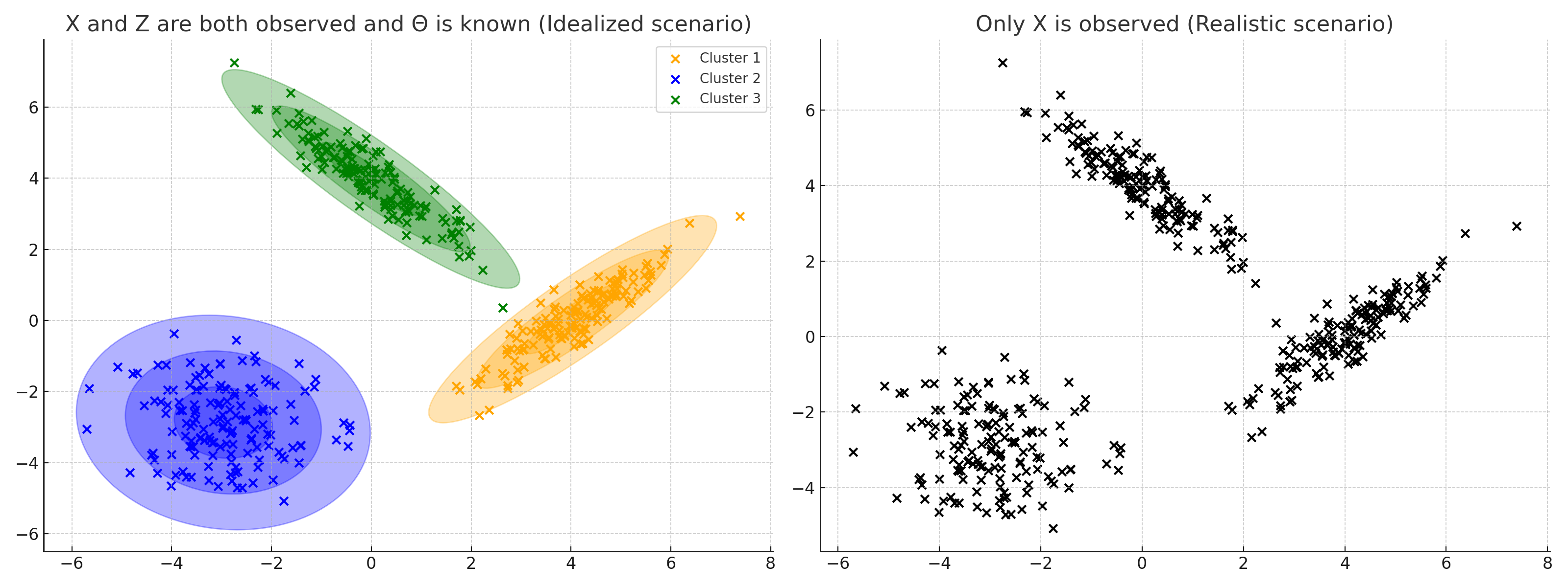
To cluster the data, we must assume that our data points were sampled from a GMM with $K$ Gaussians, where $K$ represents the number of clusters we believe accurately describe the data. However, we do not know the parameters of the GMM (i.e., the mean and covariance of each Gaussian) nor do we know which Gaussian generated each data point (i.e., the $Z_1, \ldots, Z_n$ random variables).

This scenario is illustrated in the figure below. On the left-hand side, we have a hypothetical situation where we know the GMM and the samples $x_1, \ldots, x_n$ from that model. We also know which Gaussian generated each data point—that is, we know the values $z_1, \ldots, z_n$ (these are represented by the colors of each data point). In the figure on the right, we are only provided with $x_1, \ldots, x_n$. We do not know the model’s parameters $\Theta$ nor do we know $z_1, \ldots, z_n$. In other words, $x_1, \ldots, x_n$ constitutes the observed data and $z_1, \ldots, z_n$ constitutes the latent information.

To perform clustering on the dataset $x_1, \ldots, x_n$, we follow these steps. Initially, we need to estimate the parameters for $\Theta$. The details of this estimation process are a major focus of this blog post, but for now, let’s consider that we have an estimate, denoted as:

With this estimate, we can assign each $x_i$ to the Gaussian (i.e., cluster) most likely to have generated it:

Using Bayes’ rule, we can compute this probability as follows:

We’ve only addressed a portion of the estimation challenge so far. The real task is estimating the values for $\Theta$. This can be approached using the principle of maximum likelihood:

How do we address this optimization problem? A practical and efficient method is provided by the Expectation-Maximization (EM) algorithm, which offers a step-by-step approach to iteratively improve the estimates of $\Theta$. We will explore this method in more detail later in the post.

EM algorithm for GMMs

The EM algorithm is particularly well-suited for performing maximum likelihood estimation of the parameters in Gaussian Mixture Models (GMMs) because the models involve latent variables and. For a detailed discussion of the EM algorithm, refer to my previous blog post.

The EM algorithm alternates between two main steps until convergence of the parameters is achieved. Before going deeper into the derivation, we make some notations. Let $ X := {x_1, \ldots, x_n} $ represent the collection of observed data points and $ Z := {z_1, \ldots, z_n} $ denote the collection of latent information (i.e., the information about which Gaussian generated each data point). The exected complete data log-likelihood at $ t $ where $t$ represents a specific iteration in the EM algorithm. This expected complete-data log-likelihood at the $ t $-th iteration is described in the context of the EM algorithm as follows:

This definition of the $Q(\Theta \lvert \Theta_{t})$ involves calculating the expected value of the log-likelihood of both the observed and latent data, conditioned on the observed data $X$ and the current estimate of the parameters $\Theta_{t}$. Essentially, this step assesses how well the current model parameters explain the observed data and predicts the latent variable assignments.

E-Step (Expectation Step)

During the E-step, we need to compute this expectation analytically. In the case of GMM, this expectation is derived as follows:

\(\begin{align*} Q_t(\Theta) &:= E_{Z \mid X; \Theta_t}\left[ \log p(X, Z; \Theta) \right] \\ &= \sum_{i=1}^n E_{z_i \mid \vect{x}_i; \Theta_t} \left[ \log p(\vect{x}_i, z_i ; \Theta) \right] \ \ \ \ \ \text{by the linearity of expectation} \\ &= \sum_{i=1}^n \sum_{k=1}^K P(z_i = k \mid \vect{x}_i ; \Theta_t) \log p(\vect{x}_i, z_i ; \Theta) \\ &= \sum_{i=1}^n \sum_{k=1}^K \ddfrac{P(\vect{x}_i \mid z_i = k ; \Theta_t)P(z_i = k ; \Theta_t)}{\sum_{j=1}^K P(\vect{x}_i \mid z_i = j ; \Theta_t)P(z_i = j ; \Theta_t)} \log p(\vect{x}_i, z_i ; \Theta) \\ &= \sum_{i=1}^n \sum_{k=1}^K \ddfrac{\pi_{t,k} \phi(\vect{x}_i; \vect{\mu}_{t,k}, \vect{\Sigma}_{t,k})}{\sum_{j=1}^K \pi_{t,j} \phi(\vect{x}_i; \vect{\mu}_{t,j}, \vect{\Sigma}_{t,j})} \log \pi_k \phi(\vect{x}_i ; \vect{\mu}_k, \vect{\Sigma}_k) \\ &= \sum_{i=1}^n \sum_{k=1}^K \gamma_{t, i, k} \log \pi_k \phi(\vect{x}_i ; \vect{\mu}_k, \vect{\Sigma}_k) \end{align*}\) where we denote

This step involves calculating the posterior probabilities of the latent variables given the current parameter estimates, which serve as the “responsibilities” of each Gaussian component for each data point. This posterior probabilities is of crucial as if this term is easily computed, EM algorithm will be a first tool to resort when dealing with latent variable models.

M-Step (Expectation Step)

The M-step involves optimizing the $Q(\Theta \lvert \Theta_{t})$ to determine $\Theta_{t+1}$, with the constraint that the mixture probabilities $\pi_1, \dots, \pi_K$ sum to one. This optimization is achieved using the method of Lagrange multipliers, which allows for the incorporation of the equality constraint directly into the maximization process. We formulate the Lagrangian as follows:

To find $\Theta$ that maximizes the Lagrangian, we first take the derivative with respect to $\pi_k$ and set it to zero:

Solving for $\pi_k$, we get:

Given the constraint $\sum_{k=1}^K \pi_k = 1$, we substitute and solve for $\lambda$:

This is because $\sum_{k=1}^K \gamma_{t,i,k} = 1$ for each $i$. Thus, substituting $\lambda = -n$ back, we find $\pi_k$:

This solution defines the optimal mixing probabilities based on the responsibilities $\gamma_{t,i,k}$ computed in the E-step.

Next, to update the Gaussian means $\vect{\mu}_k$, we compute the derivative of the Lagrangian with respect to $\vect{\mu}_k$ and set it to zero:

The result use the following fact:

Solving for $\vect{\mu}_k$, we find:

This calculation gives us the updated mean for each Gaussian, weighted by the responsibilities, reflecting how each data point is attributed to the respective Gaussian cluster. This step completes the parameter update for $\vect{\mu}_k$, and similar steps would follow for updating the covariance matrices $\vect{\Sigma}_k$.

To solve for the covariance matrices that maximize the Q-function, we start by computing the derivative of the Lagrangian with respect to the covariance matrix $\vect{\Sigma}_k$ for a particular $k$:

This formula uses critical insights from matrix calculus:

1. The derivative of the log determinant of $\vect{\Sigma}_k$, according to the matrix cookbook, is: \(\frac{\partial}{\partial \vect{\Sigma}_k} \log \text{det}(\vect{\Sigma}_k) = \vect{\Sigma}_k^{-1}\)

2. The derivative of the quadratic form: \(\frac{\partial}{\partial \vect{\Sigma}_k} (\vect{x}_i - \vect{\mu}_k)^T \vect{\Sigma}_k^{-1} (\vect{x}_i - \vect{\mu}_k) = -\vect{\Sigma}_k^{-1} (\vect{x}_i - \vect{\mu}_k)(\vect{x}_i - \vect{\mu}_k)^T \vect{\Sigma}_k^{-1}\)

To get the above result, let do some tedious work \(\begin{align*} \frac{\partial L(\Theta, \lambda)}{ \partial \vect{\Sigma}_k } &:= \sum_{i=1}^n \gamma_{t,i,k} \frac{\partial}{\partial \vect{\Sigma}_k } \log \pi_k \phi(\vect{x}_i ; \vect{\mu}_k, \vect{\Sigma}_k) \\ &= \sum_{i=1}^n \frac{\gamma_{t,i,k}}{\pi_k \phi(\vect{x}_i ; \vect{\mu}_k, \vect{\Sigma}_k)}\frac{\partial}{\partial \vect{\Sigma}_k} \pi_k \phi(\vect{x}_i ; \vect{\mu}_k, \vect{\Sigma}_k) \\ &= \sum_{i=1}^n \gamma_{t,i,k} \left[ -\frac{1}{2} \frac{\partial}{\partial \vect{\Sigma}_k} \log \text{det}(\vect{\Sigma_k}) - \frac{1}{2} \frac{\partial}{\partial \vect{\Sigma}_k} (\vect{x}_i - \vect{\mu}_k)^T\vect{\Sigma}_k^{-1}(\vect{x}_i - \vect{\mu}_k)\right] \\ &= \sum_{i=1}^n \gamma_{t,i,k} -\frac{1}{2}\vect{\Sigma}_k^{-1} - \gamma_{t,i,k} \frac{1}{2} \frac{\partial}{\partial \vect{\Sigma}_k} (\vect{x}_i - \vect{\mu}_k)^T\vect{\Sigma}_k^{-1}(\vect{x}_i - \vect{\mu}_k) \\ &= -\frac{1}{2}\sum_{i=1}^n \gamma_{t,i,k} \vect{\Sigma}_k^{-1} - \gamma_{t,i,k}\vect{\Sigma}_k^{-1} (\vect{x}_i - \vect{\mu}_i)(\vect{x}_i - \vect{\mu}_i)^T \vect{\Sigma}_k^{-1} \\ &= -\frac{1}{2} \left(\sum_{i=1}^n \gamma_{t,i,k}\right)\vect{\Sigma}_k^{-1} - \vect{\Sigma}_k^{-1} \left(\sum_{i=1}^n \gamma_{t,i,k} (\vect{x}_i - \vect{\mu}_i)(\vect{x}_i - \vect{\mu}_i)^T\right) \vect{\Sigma}_k^{-1}\end{align*}\)

Setting the gradient to zero and solving for $\vect{\Sigma}_k$, we get:

This result provides the update formula for the covariance matrices $\vect{\Sigma_k}$ in the M-step of the EM algorithm, ensuring that each matrix is a weighted average of the outer products of the differences between the data points and the respective cluster means, weighted by the responsibilities $\gamma_{t,i,k}$. This completes the EM algorithm’s parameter update steps for Gaussian Mixture Models.

Experiment

In this experiment, synthetic data is generated to form a scenario where Gaussian Mixture Models (GMM) can be applied to identify and analyze three distinct clusters. The data generation process involves creating three separate sets of data points, each drawn from a different multivariate normal distribution, reflecting different clusters. As you can see, as the iterations increase, the means and covariances of each Gaussian begin to shift and stretch to minimize the overlap and better capture the underlying structure of the data.

Final word

GMM algorithm can be summarized as below:

Code

The codes for running GMM and create gif are belows:

import numpy as np 
from scipy.stats import multivariate_normal
from typing import Optional, Tuple, List
import matplotlib.pyplot as plt
from matplotlib.patches import Ellipse
from matplotlib.animation import FuncAnimation
import io
from PIL import Image

class GMM:
    """
    Gaussian Mixture Model using the Expectation-Maximization algorithm.

    Parameters:
    -----------
    n_components : int, default=1
        The number of mixture components.
    max_iter : int, default=100
        The maximum number of EM iterations to perform.
    tol : float, default=1e-3
        The convergence threshold. EM iterations will stop when the lower bound average gain is below this threshold.
    random_state : Optional[int], default=None
        Controls the random seed given to the method for initialization.

    Attributes:
    -----------
    weights_ : np.ndarray, shape (n_components,)
        The weights of each mixture component.
    means_ : np.ndarray, shape (n_components, n_features)
        The mean of each mixture component.
    covariances_ : np.ndarray, shape (n_components, n_features, n_features)
        The covariance of each mixture component.
    converged_ : bool
        True when convergence was reached in fit(), False otherwise.
    """
    def __init__(self, n_components: int = 1, max_iter: int = 100, tol: float = 1e-3, random_state: Optional[int] = None):
        self.n_components = n_components
        self.max_iter = max_iter
        self.tol = tol
        self.random_state = random_state
        
        self.weights_: Optional[np.ndarray] = None
        self.means_: Optional[np.ndarray] = None
        self.covariances_: Optional[np.ndarray] = None
        self.converged_: bool = False

    def _initialize(self, X: np.ndarray) -> None:
        n_samples, n_features = X.shape
        np.random.seed(self.random_state)
        
        self.weights_ = np.full(self.n_components, 1/self.n_components)
        random_indices = np.random.choice(n_samples, self.n_components, replace=False)
        self.means_ = X[random_indices]
        self.covariances_ = np.array([np.cov(X.T) for _ in range(self.n_components)])

    def fit(self, X: np.ndarray) -> 'GMM':
        """
        Estimate model parameters with the EM algorithm.

        Parameters:
        -----------
        X : np.ndarray, shape (n_samples, n_features)
            The input data.

        Returns:
        --------
        self : GMM class
            The fitted model.
        """
        self._initialize(X)
        
        log_likelihood = -np.inf
        for iteration in range(self.max_iter):
            responsibilities = self._e_step(X)
            self._m_step(X, responsibilities)
            new_log_likelihood = self._compute_log_likelihood(X)
            
            if np.abs(new_log_likelihood - log_likelihood) < self.tol:
                self.converged_ = True
                break
            
            log_likelihood = new_log_likelihood
        
        return self

    def _e_step(self, X: np.ndarray) -> np.ndarray:
        """
        Expectation step: compute responsibilities.

        Parameters:
        -----------
        X : np.ndarray, shape (n_samples, n_features)
            The input data.

        Returns:
        --------
        responsibilities : np.ndarray, shape (n_samples, n_components)
            The responsibility of each data point to each Gaussian component.
        """
        responsibilities = np.zeros((X.shape[0], self.n_components))
        
        for k in range(self.n_components):
            responsibilities[:, k] = self.weights_[k] * multivariate_normal.pdf(X, self.means_[k], self.covariances_[k])
        
        responsibilities /= responsibilities.sum(axis=1, keepdims=True)
        return responsibilities

    def _m_step(self, X: np.ndarray, responsibilities: np.ndarray) -> None:
        """
        Maximization step: update parameters.

        Parameters:
        -----------
        X : np.ndarray, shape (n_samples, n_features)
            The input data.
        responsibilities : np.ndarray, shape (n_samples, n_components)
            The responsibility of each data point to each Gaussian component.
        """
        N = responsibilities.sum(axis=0)
        
        self.weights_ = N / X.shape[0]
        self.means_ = np.dot(responsibilities.T, X) / N[:, np.newaxis]
        
        for k in range(self.n_components):
            diff = X - self.means_[k]
            self.covariances_[k] = np.dot(responsibilities[:, k] * diff.T, diff) / N[k]

    def _compute_log_likelihood(self, X: np.ndarray) -> float:
        """
        Compute the log-likelihood of the data.

        Parameters:
        -----------
        X : np.ndarray, shape (n_samples, n_features)
            The input data.

        Returns:
        --------
        log_likelihood : float
            The log-likelihood of the data under the current model parameters.
        """
        log_likelihood = 0
        for k in range(self.n_components):
            log_likelihood += self.weights_[k] * multivariate_normal.pdf(X, self.means_[k], self.covariances_[k])
        return np.sum(np.log(log_likelihood))

    def predict(self, X: np.ndarray) -> np.ndarray:
        """
        Predict the labels for the data samples in X using trained model.

        Parameters:
        -----------
        X : np.ndarray, shape (n_samples, n_features)
            The input data.

        Returns:
        --------
        labels : np.ndarray, shape (n_samples,)
            Component labels.
        """
        responsibilities = self._e_step(X)
        return np.argmax(responsibilities, axis=1)

    def score_samples(self, X: np.ndarray) -> np.ndarray:
        """
        Compute the log-likelihood of each sample.

        Parameters:
        -----------
        X : np.ndarray, shape (n_samples, n_features)
            The input data.

        Returns:
        --------
        log_likelihood : np.ndarray, shape (n_samples,)
            Log-likelihood of each sample under the current model.
        """
        log_likelihood = 0
        for k in range(self.n_components):
            log_likelihood += self.weights_[k] * multivariate_normal.pdf(X, self.means_[k], self.covariances_[k])
        return np.log(log_likelihood)

class IterativeGMM(GMM):
    def __init__(self, *args, **kwargs):
        super().__init__(*args, **kwargs)
        self.iteration = 0

    def fit_step(self, X):
        if self.iteration == 0:
            self._initialize(X)
        
        responsibilities = self._e_step(X)
        self._m_step(X, responsibilities)
        log_likelihood = self._compute_log_likelihood(X)
        
        self.iteration += 1
        return log_likelihood

def plot_gmm_step(X, gmm, ax):
    ax.clear()
    scatter = ax.scatter(X[:, 0], X[:, 1], c='gray', alpha=0.3)
    
    if gmm.iteration > 0:
        labels = gmm.predict(X)
        scatter = ax.scatter(X[:, 0], X[:, 1], c=labels, cmap='viridis', alpha=0.7)
        
        for i in range(gmm.n_components):
            mean = gmm.means_[i]
            covar = gmm.covariances_[i]
            v, w = np.linalg.eigh(covar)
            angle = np.arctan2(w[0][1], w[0][0])
            angle = 180 * angle / np.pi
            v = 2. * np.sqrt(2.) * np.sqrt(v)
            ell = Ellipse(mean, v[0], v[1], 180 + angle, color='red', alpha=0.3)
            ax.add_artist(ell)
            ax.scatter(mean[0], mean[1], c='red', marker='x', s=100, linewidths=3)
    
    ax.set_xlim(-8, 8)
    ax.set_ylim(-6, 6)
    ax.set_title(f'Iteration {gmm.iteration}')
    return scatter

def create_gmm_gif(X, n_components, max_iter, filename='./assets/gmm_iterations.gif'):
    gmm = IterativeGMM(n_components=n_components, max_iter=max_iter, random_state=42)
    
    fig, ax = plt.subplots(figsize=(10, 8))
    scatter = plot_gmm_step(X, gmm, ax)
    
    def update(frame):
        gmm.fit_step(X)
        scatter = plot_gmm_step(X, gmm, ax)
        return scatter,
    
    anim = FuncAnimation(fig, update, frames=max_iter, interval=500, blit=False, repeat=False)
    
    anim.save(filename, writer='pillow', fps=2)
    plt.close(fig)
    
    print(f"GIF saved as '{filename}'")


# Create and save the GIF
create_gmm_gif(X, n_components=3, max_iter=30)