Binh Ho
Maximum A Posterior
It is well-known that There are two ways of evaluating parameters commonly used in statistical machine learning. The first method is based solely on known data in the training data, called Maximum Likelihood Estimation or ML Estimation or MLE. The second method is based not only on training data but also on the known information of parameters. This information can be obtained by the sense of the model builder. The clearer the senses, the more rational, the higher the likelihood of obtaining a good set of parameters. For example, in the coin tossing problem, given the parameter of interest $\theta$ being the probability of obtaining a head, we can expect this parameter’s value should be close to $0.5$. This second approach for learning and assessing parameters is called Maximum A Posteriori Estimation or MAP Estimation. Despite some differences, the mathematical structures underpinning behind the two methods forge a connection between them. In this article, I will present the idea and how to solve the problem of evaluating model parameters according to MLE or MAP Estimation. And as always, we’ll go through a few simple examples.
Maximum a Posteriori
Why needs MAP?
A key issue with MLE is that they aim to opt for parameters that minimize the loss function over the training data. However, this may not result in a model that can perform well on future data, which is called overfitting. A simple example to illustrate the failure of MLE in generalizing ability is again the coin tossing problem.
Suppose that you toss the coin $5$ times and and observe $5$ head faces, according to the MLE, the chance of attaining a head would be $\theta_{MLE} = \frac{N_{\text{head}}}{N_{\text{tail}} + N_{\text{head}}} = \frac{5}{5} = 1$. It would be too unrealistic to conclude such result since we have too little data (corresponding to the phenomenon of having too little data in training . The key issue concerned with low-training data is that the training data may not be representative for the true distribution that we are trying to inference; thereby, the perfectly fitted model on the training data may not generalize well enough when future data is coming. One common remedy to this problem is to deduce some assumptions of the parameters. For example, with a coin toss, our assumption is that the probability of getting the head should be approximately close to $0.5$.
MAP Formulation
Maximum A Posteriori (MAP) was devised to tackle this problem. In MAP, we introduce a known assumption, called a prior, of the parameter $\theta$. Based on our previous experience, we can deduce the distributions of such prior on parameters.
In constrast of MLE, which use the likelihood (in other words, the joint distribution of the data and the parameter), MAP evaluate the parameter as a conditional probability of the data:
\[\theta = \underset{\theta}{\mathrm{argmax}}\ \underbrace{P(\theta \lvert x_1, x_2, \dots, x_N)}_{\text{posterior}} \tag{1}\]The expression of the maximization problem $P(\theta \lvert x_1, x_2 \dots, x_N)$ is generally known as posterior probability of $\theta$. This is also the reason why this method is named Maximum A Posteriori.
It is easy to see the connection with the Bayesian context. Bayesian analysis commences from formulating the link between the posterior, the likelihood, the prior and the evidence. The objective of Bayesian inference is to estimate the posterior distribution (which is often intractable), by taking the product of likelihood and the prior and often ignore the evidence since it does not depend on the parameter $\theta$. Denote a random sample $(x_1, x_2, \dots, x_N)$ of a random variable $X$. Then,
\[\begin{align} \theta_{MAP} &= \mathop{\rm argmax}\limits_{\theta} P(X \vert \theta) P(\theta) \\ &= \mathop{\rm argmax}\limits_{\theta} \log P(X \vert \theta) + \log P(\theta) \\ &= \mathop{\rm argmax}\limits_{\theta} \log \prod_{i = 1}^n P(x_i \vert \theta) + \log P(\theta) \\ &= \mathop{\rm argmax}\limits_{\theta} \sum_{i = 1}^n \log P(x_i \vert \theta) + \log P(\theta) \end{align} \tag{2}\]The last expression is identical to that of MLE, except for the inclusion of the term $\log{P(\theta)}$ - the log prior of the parameter $\theta$. In simpler terms, if we define a prior distribution for the model parameter, the likelihood is influenced not only by the likelihood of each data point but also by the prior. Think of the prior as an extra “constraint” in a broad sense. The best parameter must fit the data and also not stray too far from the prior. Normally, prior is usually chosen based on the pre-known information of the parameter, and the distribution chosen is usually conjugate distributions with likelihood, i.e. distributions that cause prior multiplication to retain the same structure as likelihood.
Conjugate Prior
In Bayesian inference, conjugacy implies that the posterior $p(\theta \lvert X)$ has the same functional form as the prior $p(\theta)$. If such case occurs, we state that the prior $p(\theta)$ is conjugate to the likelihood function $p(X \lvert \theta)$. Specifically, if we look at the standard Bayes’ formula, the following terms have the same functional form
\(\boxed{p(\theta \lvert X)} = \dfrac{p(X \lvert \theta) \boxed{p(\theta)}}{\int p(X \lvert \theta^\prime) p(\theta^\prime)\, d \theta^\prime}\).
Recalling the earlier example about the bias $\theta$ of a coin. For $N$ times flips, the outcome of the $i^{\text{th}}$ coin toss is $x_i$ belonging to a Bernoulli random variable $X_i$ that takes on value of $0$ and $1$ (tail or head respectively). Then, we have shown that the maximum likelihood estimator of $\theta$, denoted by $\hat{\theta}_{MLE} = \frac{N_1}{N_1 + N_2}$ where $N_1$ and $N_2$ denotes the number of heads and tails in all tosses respectively. In low-data case, this estimator might suffer from being overfitted. One remedy is to use MAP (or Bayesian inference) to impose a constraint (in this method it is the incorporation of prior knowledge about what $\theta$ normally is into the model). The question arises on the way to sort out the prior we should place on $\theta$. Conjugate prior is the key!
Coin tossing in Bayesian paradigm
We still hold an assumption that the majority of coins is fair. Then even though we observe five heads in a row, we want to incorporate our prior knowledge of what the true probability of head typical is into our model. The remanining question lies in the choice of prior imposing on our parameter of interest $\theta$. Beginning with the two modeling assumptions made earlier. Suppose that most coins are fair. This implies that the mode of the distribution should be around $0.5$. Additionally, we assume that biased coins do not favor heads over tails. This indicates that we should choose a symmetric distribution. One distribution that may have these properties is the beta distribution, which is given by the following formula
\[\text{Beta}(\lambda \lvert \alpha, \beta) = \frac{\Gamma(\alpha + \beta)}{\Gamma(\alpha) \Gamma(\beta)} \lambda^{\alpha - 1} ( 1 - \lambda) ^{\beta - 1}. \tag{3}\]where $\Gamma(x)$ is the gamma function
\[\Gamma(x) = \int_{0}^{\infty} \lambda^{x-1} \exp{-\lambda} d\lambda.\]and the term $\frac{\Gamma(\alpha + \beta)}{\Gamma(\alpha) \Gamma(\beta)}$ is the normalization that ensures this is a proper distribution. That is, we can easily check that
\[\int_{0}^{1} \lambda^{\alpha - 1} ( 1 - \lambda) ^{\beta - 1} d\lambda = \frac{\Gamma(\alpha + \beta)}{\Gamma(\alpha) \Gamma(\beta)}.\]The first and second moments of Beta distribution are given by
\[\begin{align} \mathbb{E}[\lambda] &= \frac{\alpha}{\alpha + \beta} \\ \text{Var}[\lambda] &= \frac{\alpha \beta}{(\alpha + \beta)^2 (\alpha + \beta + 1)} \end{align}\]However, the most crucial property of the beta distribution that serves its usefulness in this Bernoulli model is that its conjugacy to the likelihood function. That is, if we ignore the constant factorization for the purpose of normalizing the integral of the probability density function equal to $1$, we can see that the rest of the beta distribution is in the same family as the Bernoulli distribution. Denoted the number of failures in terms of successes by $n_2 = n - n_1$. If we multiply our likelihood given by
\[\begin{align} P(\mathcal{D} \lvert \theta) &= \prod_{i = 1}^n P(x_i \vert \theta) \\ &= \prod_{i = 1}^n {n \choose n_1} \theta^{x_i} (1 - \theta)^{(1- x_i)} \\ &= {n \choose n_1} \theta^{n_1} (1- \theta)^{(n - n_1)} \end{align}\]by Equation (3), we obtain the posterior distribution that has the same functional form as the prior
\[\begin{align} P(\theta \lvert n_1, n_2, \alpha, \beta) &= \frac{\Gamma(\alpha + \beta)}{\Gamma(\alpha) \Gamma(\beta)} \lambda^{\alpha - 1} ( 1 - \lambda) ^{\beta - 1} \prod_{i = 1}^n {n \choose n_1} \theta^{x_i} (1 - \theta)^{(1- x_i)} \\ &\propto \theta^{n_1 + \alpha - 1} (1-\theta)^{n_2 + \beta - 1} \end{align}\]Note that we are only interested in terms that include $\theta$ since it is our learning parameter; thereby, we care about proportionality and drop constant terms. The conjugate Beta prior combined with the Binomial data model yield a Beta posterior model for $\theta$ with the updated distribution
\[P(\theta \lvert n_1, n_2, \alpha, \beta) = \frac{\Gamma(n_1 + \alpha + n_2 + \beta)}{\Gamma(n_1 + \alpha) \Gamma(n_2 + \beta)} \theta^{(n_1 + \alpha -2)} (1 - \theta)^{(n_2 +\beta -1)}. \tag{4}\]Finally, our MAP optimization problem involves with optimizing Equation (4)
\[\mathop{\rm argmax}\limits_{\theta} \left[ \lambda^{n_1 + \alpha - 1} ( 1- \lambda)^{n_2 + \beta - 1} \right] \tag{5}\]Computing the derivatiove of the log of the objective function with respect to $\theta$ in (5)
\[\frac{\partial}{\partial \theta} \log P(\theta \lvert n_1, n_2, \alpha, \beta) = \frac{n_1 + a - 1}{\theta} - \frac{n_2 + \beta - 1}{1- \theta}.\]Setting this equal to 0 and algebraically manipulating, we arrive at
\[\theta_{\text{MAP}} = \frac{n_1 + \alpha -1}{n + \alpha + \beta - 2} \tag{6}\]If $n_1 = n = 0$ or in other words, we do not conduct any flips to estimate the probability of head, the best and most reasonable we can do is assuming this probability of head to be the mode of our prior (it means we believe entirely in our knowledge).
Earlier, I’ve said that based on assumption most of our coins are fair or the mode of our prior distribution should be $0.5$. At this step, the only thing we need to do is to opt for an appropriate pair of $(\alpha, \beta)$ to match with our belief. Let’s review the shape of the beta distribution and notice that when $\alpha = \beta > 1$, we have the probability density function of the symmetric Beta distribution through the point 0.5 and reach the highest value at $0.5$. Consider the Figure 1, we notice that when we increase the value of $\alpha = \beta$, the mode of Beta distribution is more centered around $0.5$.
If we choose $\alpha = \beta = 1$, we see that the prior is uniform since the density function is a straight line. Therefore, we place the chance of $\theta$ at every point in the interval $[0,1]$ equally. In fact, if we plug in the uniform prior into Equation (6) we obtain the normal MLE $\theta = \frac{n_1}{n}$. We can conclude that MLE is a special case of MAP when the prior is a uniform distribution.
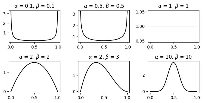
Turning back to our supposition, we should choose $\alpha = \beta > 1$ to be in harmony with our analysis. If $\alpha = \beta = 2$, we obtain
\[\theta = \frac{n_1 + 1}{n + 2}\]For example, when $n=5, n_1 = 5$ as in the earlier example, MLE results in $\theta = 1$, while MAP will raise $\theta = \frac{6}{7}$. If we select a larger value for $\alpha = \beta$, the more we get $\theta$ as close as possible to $0.5$. This is due to the fact that our data in this case is less influenced than our belief; hence, the impact of the observing data is negligible.
In conclusion, we have demonstrated why the prior (or regularization term) is extremely beneficial and important for parameter estimation with small data and the way it helps avoid overfitting.