Bootstrapping intermittent demand with a Markov chain

Intermittent demand is demand that is zero in most periods and positive, with variable size, in the others. Spare parts, slow-moving retail items and many products in large inventories behave this way. Standard forecasting models for continuous, smoothly varying series fit such data poorly, and the classical alternative, Croston’s method (Croston, 1972), forecasts the mean demand per period by smoothing the sizes and the intervals between demands separately. For inventory control, however, the mean is not the quantity of interest. What matters is the distribution of the total demand over the replenishment lead time, since a reorder point that achieves a 95% service level is the 0.95 quantile of that distribution.

Willemain, Smart and Schwarz (2004) proposed a bootstrap that targets this distribution directly. It modifies the ordinary bootstrap of Efron (1979) in two ways: a Markov chain carries the serial dependence between periods with and without demand, and a “jittering” step allows demand sizes that did not occur in the history. Below I describe the method, give an implementation in R, check it on simulated data for which the true lead-time distribution is known, and derive the maximum likelihood estimator of the transition probabilities that the method uses.

Why the ordinary bootstrap is not enough

Let $y_1, \dots, y_n$ be the observed demands, nonnegative integers. The ordinary bootstrap would build a lead-time demand replicate by drawing $L$ values independently and with replacement from $\{y_1, \dots, y_n\}$ and adding them. This has two defects for intermittent series.

It destroys serial dependence. Demand occurrence is often autocorrelated: periods with demand tend to cluster, or, for items bought in single large orders, to repel each other. Independent resampling treats the periods as exchangeable. It reproduces the long-run mean of the lead-time total, but it ignores the current state of the series and gets the spread wrong.
It reproduces only observed values. Every resampled demand size is a value already seen. With a short history, sizes that are plausible but happened not to occur get probability zero, and the upper tail of the lead-time distribution is cut off.

The method addresses the first defect with a Markov chain and the second by jittering.

The method

Write $I_t = \mathbf 1\{y_t > 0\}$ for the demand indicator. The occurrence process $(I_t)$ is modelled as a two-state Markov chain with transition probabilities

\[p_{01} = \P(I_t = 1 \mid I_{t-1} = 0), \qquad p_{11} = \P(I_t = 1 \mid I_{t-1} = 1),\]

and $p_{00} = 1 - p_{01}$, $p_{10} = 1 - p_{11}$. The demand sizes in periods with demand are treated as draws from the distribution of the positive values in the history, independent of the occurrence process. One bootstrap replicate of the demand over the next $L$ periods is generated as follows.

Estimate the transition probabilities from the observed indicators $I_1, \dots, I_n$ by maximum likelihood: $\hat p_{ij}$ is the number of transitions from $i$ to $j$ divided by the number of transitions out of $i$ (derived in the appendix).
Starting from the last observed state $I_n$, simulate $I_{n+1}, \dots, I_{n+L}$ from the estimated chain.
For each simulated period with $I_{n+h} = 1$, draw a size $X^\ast$ uniformly at random from the positive demands $\{y_t : y_t > 0\}$, counted with their multiplicities.
Jitter the size: with $Z \sim N(0, 1)$ independent of everything else, set
\[X = \begin{cases} 1 + \operatorname{int}\bigl(X^\ast + Z\sqrt{X^\ast}\bigr) & \text{if this value is positive,} \\ X^\ast & \text{otherwise,} \end{cases}\]
where $\operatorname{int}$ denotes the integer part (truncation towards zero). Periods with $I_{n+h} = 0$ get demand $0$.
Sum the $L$ simulated demands.

Repeating the steps $B$ times gives $B$ draws from the estimated lead-time demand distribution. Its empirical quantiles serve as reorder points, and the average of the replicates for each future period gives per-period point forecasts if those are needed.

The jittering step has two properties that affect the output. Its spread is of order $\sqrt{X^\ast}$, as for a Poisson count with mean $X^\ast$, so large sizes are perturbed more than small ones, and the rule never produces a nonpositive size. It is not mean-preserving, however: for moderate $X^\ast$, the integer part loses about one half on average and the added one more than compensates, so the jittered size exceeds $X^\ast$ by roughly $1/2$ on average (by simulation, about $0.58$ for $X^\ast = 3$ and $0.50$ for $X^\ast = 10$). Rounding $X^\ast + Z\sqrt{X^\ast}$ to the nearest integer instead of applying $1 + \operatorname{int}(\cdot)$ removes the shift for large sizes (it is about $0.01$ at $X^\ast = 10$) but not for small ones, where replacing nonpositive values by $X^\ast$ still raises the mean (by about $0.25$ at $X^\ast = 3$). The code below follows the published rule.

What the Markov chain captures

The effect of the chain on the spread of the lead-time demand can be computed exactly for the number of demand occurrences $N_L = \sum_{h=1}^L I_{n+h}$. For a two-state chain with $0 < p_{01} + p_{10} < 2$, the stationary probability of demand is $\pi = p_{01}/(p_{01} + p_{10})$, and the chain has second eigenvalue $\kappa = 1 - p_{01} - p_{10} = p_{11} - p_{01}$. In stationarity, $\P(I_{t+h} = 1 \mid I_t = 1) = \pi + (1-\pi)\kappa^h$, which gives the autocovariance $\Cov(I_t, I_{t+h}) = \pi(1-\pi)\kappa^h$, and therefore

\[\Var(N_L) = L\pi(1-\pi)\Bigl\{1 + 2\sum_{h=1}^{L-1}\Bigl(1 - \frac hL\Bigr)\kappa^h\Bigr\}.\]

Independent resampling corresponds to $\kappa = 0$. When occurrences cluster ($\kappa > 0$), the factor in braces exceeds one and the independent bootstrap understates the variance; when they repel ($\kappa < 0$), it overstates it. In the simulation below, $p_{01} = 0.1$ and $p_{11} = 0.6$, so $\pi = 0.2$, $\kappa = 0.5$, and for $L = 12$ the factor is $2.67$: clustering multiplies the variance of the number of demand periods by more than two and a half.

Implementation

The following base R functions implement the method. The data are a vector y of nonnegative integer demands; the output is a $B \times h$ matrix of simulated demand paths.

fit_occurrence_chain <- function(y) {
  s <- as.integer(y > 0)                 # 0 = no demand, 1 = demand
  n <- table(factor(head(s, -1), levels = 0:1),
             factor(tail(s, -1), levels = 0:1))   # counts n_ij
  if (any(rowSums(n) == 0)) stop("a state is never left")
  unclass(n / rowSums(n))                # MLE: row-normalized counts
}

wss_bootstrap <- function(y, h, B = 5000) {
  P <- fit_occurrence_chain(y)
  sizes <- y[y > 0]                      # positive demands, repeats kept
  out <- matrix(0, B, h)
  for (b in seq_len(B)) {
    state <- as.integer(y[length(y)] > 0)  # last observed state
    for (t in seq_len(h)) {
      state <- rbinom(1, 1, P[state + 1, 2])
      if (state == 1) {
        x <- sizes[sample.int(length(sizes), 1)]
        xj <- 1 + trunc(x + sqrt(x) * rnorm(1))   # jittering
        out[b, t] <- if (xj > 0) xj else x
      }
    }
  }
  out
}

paths <- wss_bootstrap(y, h = 12, B = 5000)
lead_time <- rowSums(paths)
quantile(lead_time, c(0.50, 0.90, 0.95))   # candidate reorder points

Two details matter in R. Sizes are drawn with sample.int on the index, because sample(x, 1) with a vector x of length one samples from 1:x instead. And the sizes are resampled with their multiplicities; removing duplicates with unique would give every distinct size the same probability and distort the size distribution. The transition probabilities can equally be estimated with markovchainFit from the markovchain package, whose default method computes the same maximum likelihood estimate. Its predict method, however, returns the most probable sequence of states, a deterministic path, and cannot replace the simulation in step 2.

In an earlier version of this note I applied the method to the daily sales of one item from the M5 forecasting competition data. Here I use a simulated series instead, so that the true lead-time distribution is available for comparison.

A simulation

The history consists of $n = 730$ periods (two years of daily data) from the model above: occurrences follow the Markov chain with $p_{01} = 0.1$ and $p_{11} = 0.6$, started from its stationary distribution, and each positive demand is $1 + \mathrm{Poisson}(3)$. The last observed period has no demand. The true distribution of the total demand over the next $L = 12$ periods given this last state is computed by simulating the true model; the Markov bootstrap and the ordinary bootstrap are computed from the history alone, each with $B = 20{,}000$ replicates.

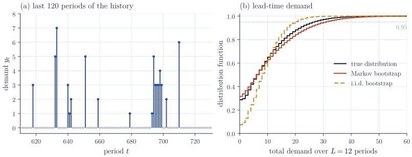
Simulated intermittent demand series and distribution functions of lead-time demand under the true model, the Markov bootstrap and the i.i.d. bootstrap — Figure 1. (a) The last 120 of 730 simulated periods; occurrences follow a two-state Markov chain with $p_{01} = 0.1$, $p_{11} = 0.6$, and positive demands are $1 + \mathrm{Poisson}(3)$. (b) Distribution functions of the total demand over the next $L = 12$ periods: the true conditional distribution given the last state, the Markov bootstrap with jittering, and the ordinary bootstrap that resamples periods independently. The dotted line marks the 0.95 level.

The ordinary bootstrap gets the centre of the distribution roughly right (mean $9.1$ against a true $8.7$), but its spread is far too small: standard deviation $6.0$ against $9.1$, a probability of zero demand of $0.07$ against $0.29$, and a 0.95 quantile of $20$ against $27$. A reorder point set from it would run out of stock much more often than the nominal 5% of cycles. The Markov bootstrap reproduces the shape, including the atom at zero ($0.32$), and its 0.95 quantile of $31$ errs on the conservative side. Its mean of $9.5$ is somewhat too high, partly because of sampling error in the estimated transition probabilities and partly because of the upward shift of the jittering rule discussed above.

Appendix: maximum likelihood for a Markov chain

Let $X_1, \dots, X_n$ be a Markov chain on the finite state space $S = \{1, \dots, m\}$ with transition matrix $P = (p_{ij})$, whose rows are probability vectors, and let $x_1, \dots, x_n$ be the observed path. By the definition of conditional probability and the Markov property, $\P(X_t = x_t \mid X_1 = x_1, \dots, X_{t-1} = x_{t-1}) = p_{x_{t-1} x_t}$, so

\[\P(X_1 = x_1, \dots, X_n = x_n) = \P(X_1 = x_1) \prod_{t=2}^n p_{x_{t-1} x_t}.\]

We treat the initial distribution as unrelated to $P$ and work with the likelihood conditional on $X_1 = x_1$. Let $n_{ij}$ be the number of indices $t \in \{2, \dots, n\}$ with $x_{t-1} = i$ and $x_t = j$, and $n_{i\cdot} = \sum_j n_{ij}$ the number of transitions out of $i$, that is, the number of visits to $i$ among $x_1, \dots, x_{n-1}$. Grouping equal factors,

\[\ell(P) = \sum_{t=2}^n \log p_{x_{t-1} x_t} = \sum_{i=1}^m \sum_{j=1}^m n_{ij} \log p_{ij},\]

with the convention $0 \log 0 = 0$.

Proposition 1. Every maximizer of $\ell$ over the set of transition matrices satisfies

\[\hat p_{ij} = \frac{n_{ij}}{n_{i\cdot}} \qquad \text{for every } i \text{ with } n_{i\cdot} > 0 \text{ and every } j .\]

Rows with $n_{i\cdot} = 0$ do not enter $\ell$ and are not determined by the data.

Proof. The log-likelihood is a sum of terms $\ell_i(p_{i\cdot}) = \sum_j n_{ij}\log p_{ij}$, each depending only on row $i$, and the constraints act row by row, so the rows can be maximized separately. Fix $i$ with $n_{i\cdot} > 0$ and write $\hat p_{ij} = n_{ij}/n_{i\cdot}$. For any probability vector $(p_{i1}, \dots, p_{im})$ with $\ell_i > -\infty$, which requires $p_{ij} > 0$ whenever $n_{ij} > 0$,

\[\ell_i(\hat p_{i\cdot}) - \ell_i(p_{i\cdot}) = n_{i\cdot} \sum_{j : n_{ij} > 0} \hat p_{ij} \log \frac{\hat p_{ij}}{p_{ij}} = n_{i\cdot}\, \KL(\hat p_{i\cdot} \,\Vert\, p_{i\cdot}) \ge 0 ,\]

where the sum is the Kullback–Leibler divergence between the two probability vectors (terms with $\hat p_{ij} = 0$ contribute nothing). By Gibbs’ inequality the divergence vanishes only if $p_{i\cdot} = \hat p_{i\cdot}$, so $\hat p_{i\cdot}$ is the unique maximizer of $\ell_i$.

The same answer comes out of Lagrange multipliers, or of eliminating one probability per row through $p_{i1} = 1 - \sum_{j \ge 2} p_{ij}$ and setting the partial derivatives $n_{ij}/p_{ij} - n_{i1}/p_{i1}$ to zero, which shows that $n_{ij}/p_{ij}$ is constant in $j$ and hence $p_{ij} \propto n_{ij}$. Both routes find a stationary point and need concavity or a boundary check to conclude; the divergence argument handles zero counts and gives uniqueness at once.

For a row that is never left, typically a state that occurs only at the last time point, any convention is consistent with the data, such as an absorbing row ($\hat p_{ii} = 1$) or a uniform one. In short series a more useful remedy is smoothing: adding a pseudo-count $a > 0$ to every $n_{ij}$ gives $(n_{ij} + a)/(n_{i\cdot} + ma)$, the posterior mean under independent Dirichlet$(a, \dots, a)$ priors on the rows, which is never zero.

If the chain is irreducible, the ergodic theorem for Markov chains gives $n_{ij}/n \to \pi_i p_{ij}$ and $n_{i\cdot}/n \to \pi_i$ almost surely, where $\pi$ is the stationary distribution and $\pi_i > 0$ for every $i$. Hence $\hat p_{ij} \to p_{ij}$ almost surely as $n \to \infty$, whatever the initial state. Asymptotic normality of the estimated rows, with multinomial covariance and independence across rows, goes back to Anderson and Goodman, “Statistical inference about Markov chains” (Annals of Mathematical Statistics, 1957).

References

Croston, J. D. (1972). Forecasting and stock control for intermittent demands. Operational Research Quarterly, 23, 289–303.
Efron, B. (1979). Bootstrap methods: another look at the jackknife. Annals of Statistics, 7, 1–26.
Willemain, T. R., Smart, C. N. and Schwarz, H. F. (2004). A new approach to forecasting intermittent demand for service parts inventories. International Journal of Forecasting, 20, 375–387.
Shalizi, C. R. Lecture notes on maximum likelihood estimation for Markov chains, Carnegie Mellon University, course 36-462, on which the appendix was originally based.