Variational inference and the evidence lower bound
Bayesian inference requires the posterior distribution of the unknown quantities given the data, and the posterior involves an integral that is rarely available in closed form. Markov chain Monte Carlo methods approximate the posterior by simulation. They are asymptotically exact, but they can be slow to converge for large data sets or strongly dependent posteriors, and assessing their convergence is itself a statistical problem. Variational inference takes a different route: it chooses a family of tractable distributions and finds the member closest to the posterior in Kullback–Leibler divergence. Integration is replaced by optimization, which is usually faster and scales to large problems, at the price of an approximation error that does not vanish with more computation.
The central object is the evidence lower bound, or ELBO. Below I derive it in two ways, identify the gap between the bound and the log evidence, and work out coordinate ascent for mean-field families, including an example in which every quantity can be computed exactly.
Setting
Let \(x\) denote the observed data and \(z \in \mathcal Z\) the unobserved quantities, which may include both parameters and latent variables. A Bayesian model specifies a joint density \(p(x, z) = p(x \mid z)\, p(z)\) with respect to a reference measure \(\dd z\) on \(\mathcal Z\) (Lebesgue measure, counting measure, or a product of the two). The posterior density is
\[p(z \mid x) = \frac{p(x, z)}{p(x)}, \qquad p(x) = \int_{\mathcal Z} p(x, z)\, \dd z ,\]and we assume throughout that \(0 < p(x) < \infty\). The normalizing constant \(p(x)\) is the evidence, or marginal likelihood: the density of the observed data under the model, with the unknowns averaged over the prior. It is a number for fixed \(x\), not a function of any parameter. Its value measures how well the model as a whole predicted the data, which is why ratios of evidences, Bayes factors, are used to compare models. The difficulty is that \(p(x)\) is an integral over \(\mathcal Z\), often high-dimensional, of a function that can be evaluated pointwise but not integrated analytically. Without \(p(x)\) the posterior is known only up to a constant, which is enough for some purposes (finding its mode, running a Metropolis–Hastings sampler) but not for computing posterior expectations or probabilities.
For two densities \(q\) and \(r\) on \(\mathcal Z\), the Kullback–Leibler divergence is
\[\KL(q \,\Vert\, r) = \int_{\mathcal Z} q(z) \log \frac{q(z)}{r(z)}\, \dd z ,\]with the conventions \(0 \log(0/r) = 0\) and \(\KL(q \,\Vert\, r) = \infty\) if \(q\) puts positive mass where \(r = 0\). Variational inference fixes a family \(\mathcal Q\) of densities on \(\mathcal Z\) and seeks
\[q^\ast \in \argmin_{q \in \mathcal Q} \KL\bigl(q \,\Vert\, p(\cdot \mid x)\bigr).\]This objective cannot be evaluated directly, because it involves \(p(z \mid x)\) and therefore \(p(x)\). The ELBO removes the obstacle.
The evidence lower bound
Lemma 1 (Gibbs’ inequality). For densities \(q\) and \(r\) on \(\mathcal Z\), \(\KL(q \,\Vert\, r) \ge 0\), with equality if and only if \(q = r\) almost everywhere.
Proof. We may assume \(\KL(q \,\Vert\, r) < \infty\), so that \(r > 0\) wherever \(q > 0\), up to a null set. Let \(Z \sim q\) and \(W = r(Z)/q(Z)\), which is positive almost surely and satisfies \(\E W = \int_{\{q > 0\}} r(z)\, \dd z \le 1\). Since the logarithm is concave, Jensen’s inequality gives
\[-\KL(q \,\Vert\, r) = \E \log W \le \log \E W \le 0 .\]Equality in the first step requires \(W\) to be almost surely constant, by strict concavity, and equality in the second requires \(\E W = 1\). Together they give \(r = q\) on \(\{q > 0\}\) and \(\int_{\{q > 0\}} r = 1\), so \(r = q\) almost everywhere.
Here Jensen’s inequality is used in the following form: if \(W\) is an integrable random variable taking values in an interval \(I\) and \(\varphi : I \to \R\) is concave, then \(\E \varphi(W)\) is well defined in \([-\infty, \infty)\) and \(\E \varphi(W) \le \varphi(\E W)\). For a strictly concave \(\varphi\) and \(\E\varphi(W) > -\infty\), equality holds only if \(W\) is almost surely constant.
Define, for a density \(q\) on \(\mathcal Z\),
\[\mathrm{ELBO}(q) = \E_q\bigl[\log p(x, Z)\bigr] - \E_q\bigl[\log q(Z)\bigr], \qquad Z \sim q .\]Proposition 2. Suppose \(\E_q \abs{\log p(x, Z)} < \infty\) and \(\E_q \abs{\log q(Z)} < \infty\). Then
\[\log p(x) = \mathrm{ELBO}(q) + \KL\bigl(q \,\Vert\, p(\cdot \mid x)\bigr).\]Consequently \(\mathrm{ELBO}(q) \le \log p(x)\), with equality if and only if \(q = p(\cdot \mid x)\) almost everywhere.
Proof. The first integrability condition implies \(p(x, Z) > 0\) almost surely, so \(\log p(Z \mid x) = \log p(x, Z) - \log p(x)\) is finite almost surely and integrable under \(q\). By linearity of the expectation,
\[\KL\bigl(q \,\Vert\, p(\cdot \mid x)\bigr) = \E_q\bigl[\log q(Z) - \log p(x, Z) + \log p(x)\bigr] = -\mathrm{ELBO}(q) + \log p(x).\]The remaining statements follow from Lemma 1.
The identity has two readings. Since \(\log p(x)\) does not depend on \(q\), maximizing the ELBO over \(\mathcal Q\) is the same as minimizing the divergence from \(q\) to the posterior, and the ELBO involves only the joint density \(p(x, z)\), which can be evaluated. And the ELBO is a lower bound on the log evidence, whose slack is exactly the divergence: the better the approximation, the tighter the bound. This is why the maximized ELBO is often used as a surrogate for \(\log p(x)\) in model comparison, with the caveat that the slack differs from model to model.
Writing \(p(x, z) = p(x \mid z)\, p(z)\) gives a second useful form,
\[\mathrm{ELBO}(q) = \E_q\bigl[\log p(x \mid Z)\bigr] - \KL\bigl(q \,\Vert\, p(\cdot)\bigr),\]an expected log-likelihood that rewards fitting the data, minus a divergence from the prior that penalizes moving away from it.
A second derivation: Jensen’s inequality
The bound can also be obtained without reference to the posterior. Let \(q\) be any density on \(\mathcal Z\) and \(Z \sim q\). Then
\[p(x) = \int_{\mathcal Z} p(x, z)\, \dd z \ge \int_{\{q > 0\}} q(z)\, \frac{p(x, z)}{q(z)}\, \dd z = \E_q\Bigl[\frac{p(x, Z)}{q(Z)}\Bigr],\]with equality when \(q > 0\) wherever \(p(x, \cdot) > 0\). The random variable \(p(x, Z)/q(Z)\) is nonnegative with finite mean, and Jensen’s inequality for the concave logarithm gives
\[\log p(x) \ge \log \E_q\Bigl[\frac{p(x, Z)}{q(Z)}\Bigr] \ge \E_q\Bigl[\log \frac{p(x, Z)}{q(Z)}\Bigr] = \mathrm{ELBO}(q),\]where the last equality uses the integrability conditions of Proposition 2. This derivation explains the name, a lower bound on the log evidence, but by itself it says nothing about the size of the gap. Proposition 2 identifies it: the total gap \(\log p(x) - \mathrm{ELBO}(q)\), the sum of the losses in the two inequalities above, equals \(\KL(q \,\Vert\, p(\cdot \mid x))\). Both losses vanish exactly when \(q\) is the posterior: the first requires \(q > 0\) almost everywhere on \(\{p(x, \cdot) > 0\}\), and the second requires \(p(x, Z)/q(Z)\) to be almost surely constant.
Mean-field families and coordinate ascent
The choice of \(\mathcal Q\) governs both the quality of the approximation and the difficulty of the optimization. The most common choice is the mean-field family: partition \(z = (z_1, \dots, z_m)\) into blocks and take
\[\mathcal Q = \Bigl\{ q : q(z) = \prod_{j=1}^m q_j(z_j) \Bigr\},\]with each \(q_j\) an arbitrary density on the range of \(z_j\). The family discards all posterior dependence between blocks and nothing else. For fixed \(q_{-j} = \prod_{k \ne j} q_k\), write \(\E_{-j}\) for the expectation over \(z_{-j} \sim q_{-j}\).
Proposition 3 (coordinate update). Fix \(q_k\) for \(k \ne j\). Suppose that \(g_j(z_j) = \E_{-j}\bigl[\log p(x, z_j, Z_{-j})\bigr]\) is finite for almost every \(z_j\) and that \(C_j = \int \exp\{g_j(z_j)\}\, \dd z_j < \infty\). Among densities \(q_j\) for which the ELBO is finite, the ELBO is maximized uniquely by
\[q_j^\ast(z_j) = \frac{\exp\bigl\{\E_{-j} \log p(x, z_j, Z_{-j})\bigr\}}{C_j}.\]Proof. Under the product form, \(\E_q \log q(Z) = \sum_k \E_{q_k} \log q_k(Z_k)\), and by iterated expectation \(\E_q \log p(x, Z) = \E_{q_j}\, g_j(Z_j)\). Collecting the terms that involve \(q_j\),
\[\mathrm{ELBO}(q) = \E_{q_j}\bigl[g_j(Z_j) - \log q_j(Z_j)\bigr] + \text{const} = -\KL(q_j \,\Vert\, q_j^\ast) + \log C_j + \text{const},\]where the constants do not depend on \(q_j\). By Lemma 1 the right-hand side is maximized exactly at \(q_j = q_j^\ast\).
Coordinate ascent variational inference (CAVI) cycles through \(j = 1, \dots, m\), replacing \(q_j\) by \(q_j^\ast\) each time. No update decreases the ELBO, and the ELBO is bounded above by \(\log p(x)\), so the sequence of ELBO values converges. The limit need not be the global maximum over \(\mathcal Q\): the ELBO is in general not jointly concave in \((q_1, \dots, q_m)\), and different starting points can lead to different fixed points of the updates. In conditionally conjugate models, such as mixtures with conjugate priors, \(q_j^\ast\) belongs to a known exponential family, and each update reduces to computing a few expected sufficient statistics.
The procedure has the same structure as the EM algorithm, which is coordinate ascent on the same functional, \(\E_q \log p(x, Z \mid \theta) - \E_q \log q(Z)\), with the latent variables given a distribution \(q\) and the parameter \(\theta\) treated as a fixed unknown; see the note on the EM algorithm.
A Gaussian example
When the target is itself Gaussian, every step can be done by hand, and the example shows what mean-field approximation loses. Let the posterior be \(N_d(\mu, \Sigma)\) with precision matrix \(\Lambda = \Sigma^{-1}\). This is the exact posterior of the coefficients in a linear regression with Gaussian errors of known variance and a Gaussian prior, and approximately the posterior of a regular parametric model with many observations. Then \(\log p(x, z) = -\tfrac12 (z - \mu)^\top \Lambda (z - \mu) + \text{const}\).
Take each block to be one coordinate. With \(m_k\) the mean of \(q_k\), the function in Proposition 3 is, as a function of \(z_j\),
\[g_j(z_j) = -\frac{\Lambda_{jj}}{2} (z_j - \mu_j)^2 - (z_j - \mu_j) \sum_{k \ne j} \Lambda_{jk} (m_k - \mu_k) + \text{const},\]because the cross terms are linear in each \(z_k\) and the expectation of a product of independent coordinates factors. Completing the square,
\[q_j^\ast = N\Bigl(\mu_j - \frac{1}{\Lambda_{jj}} \sum_{k \ne j} \Lambda_{jk} (m_k - \mu_k),\; \frac{1}{\Lambda_{jj}}\Bigr).\]The update of the mean is the conditional mean \(\E[z_j \mid z_{-j} = m_{-j}]\) of the target, and CAVI on the means is the Gauss–Seidel iteration for the linear system \(\Lambda(m - \mu) = 0\), which converges to \(m = \mu\) from any starting point because \(\Lambda\) is positive definite. The variances are set after one update and never change.
Proposition 4. Over all product densities \(q = \prod_j q_j\) on \(\R^d\), the divergence \(\KL(q \,\Vert\, N_d(\mu, \Sigma))\) is minimized uniquely by \(q^\ast = \prod_j N(\mu_j, 1/\Lambda_{jj})\), and
\[\KL\bigl(q^\ast \,\Vert\, N_d(\mu, \Sigma)\bigr) = \frac12 \log\Bigl(\det\Sigma \prod_{j=1}^d \Lambda_{jj}\Bigr) \ge 0 .\]Proof. Write \(p\) for the target density and let \(q\) be a product density with \(\KL(q \,\Vert\, p) < \infty\). Then \(q\) has finite second moments: the Donsker–Varadhan inequality \(\E_q f(Z) \le \KL(q \,\Vert\, p) + \log \E_p e^{f(Z)}\) with \(f(z) = c\norm{z - \mu}^2\) and \(c > 0\) small enough that \(\E_p e^{f(Z)} < \infty\) bounds \(\E_q \norm{Z - \mu}^2\). Let \(m_j\) and \(v_j\) be the mean and variance of \(q_j\). By independence of the coordinates under \(q\),
\[\E_q (Z - \mu)^\top \Lambda (Z - \mu) = \sum_j \Lambda_{jj} v_j + (m - \mu)^\top \Lambda (m - \mu),\]so, writing \(H(q_j) = -\E_{q_j} \log q_j\) for the differential entropy,
\[\KL(q \,\Vert\, p) = -\sum_j H(q_j) + \frac12 \sum_j \Lambda_{jj} v_j + \frac12 (m - \mu)^\top \Lambda (m - \mu) + \frac d2 \log(2\pi) + \frac12 \log\det\Sigma .\]Among densities with variance \(v_j\), the normal density maximizes the entropy, with \(H = \tfrac12\log(2\pi e v_j)\), so replacing each \(q_j\) by a normal with the same mean and variance lowers the divergence unless \(q_j\) is already normal. It remains to minimize \(\sum_j \{-\tfrac12 \log v_j + \tfrac12 \Lambda_{jj} v_j\} + \tfrac12 (m - \mu)^\top\Lambda(m - \mu)\), which gives \(v_j = 1/\Lambda_{jj}\) and \(m = \mu\). Substituting yields the stated value, which is nonnegative by Hadamard’s inequality \(\det\Lambda \le \prod_j \Lambda_{jj}\) for positive definite \(\Lambda\).
Two features are typical of mean-field variational inference. The mean is recovered exactly, but the variances are too small: \(1/\Lambda_{jj}\) is the conditional variance \(\Var(z_j \mid z_{-j})\), which is at most the marginal variance \(\Sigma_{jj}\), with equality only when \(z_j\) is uncorrelated with the other coordinates. And the gap between the ELBO and the log evidence does not close. For two coordinates with unit variances and correlation \(\rho\), the optimal variances are \(1 - \rho^2\) and the gap is \(-\tfrac12 \log(1 - \rho^2)\).
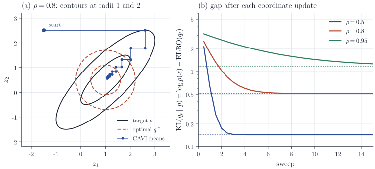
The figure also shows the cost of correlation for the optimization. In the bivariate case the mean update is \(m_1 \leftarrow \mu_1 + \rho(m_2 - \mu_2)\), followed by \(m_2 \leftarrow \mu_2 + \rho(m_1 - \mu_1)\), so each full sweep multiplies the error in the means by \(\rho^2\) and the excess divergence by \(\rho^4\). For \(\rho = 0.95\) this is about \(0.81\) per sweep, and the iteration crawls along the narrow ridge of the target.
Remarks
The direction of the divergence matters. Minimizing \(\KL(q \,\Vert\, p)\) penalizes \(q\) heavily for putting mass where \(p\) is small, so the optimal \(q\) tends to be too concentrated, as in Proposition 4, and on multimodal posteriors it tends to settle on a single mode; see the note on reverse Kullback–Leibler divergence. Minimizing \(\KL(p \,\Vert\, q)\) instead leads to moment matching and to expectation propagation. Beyond conditionally conjugate models, the ELBO is maximized by stochastic gradient methods, using Monte Carlo estimates of its gradient, which extends variational inference to models where the coordinate updates of Proposition 3 are not available in closed form.
Good starting points are Blei, Kucukelbir and McAuliffe, “Variational inference: a review for statisticians” (Journal of the American Statistical Association, 2017), Chapter 10 of Bishop, Pattern Recognition and Machine Learning, and Wainwright and Jordan, “Graphical models, exponential families, and variational inference” (Foundations and Trends in Machine Learning, 2008).