Zero-forcing: how the reverse Kullback–Leibler divergence locks onto one mode

Variational inference replaces an intractable density $p$, usually a posterior, by the member of a tractable family $\mathcal Q$ that minimizes $\mathrm{KL}(q\Vert p)$. The order of the arguments is dictated by computation: the expectation is taken under $q$, which we can sample from, and $p$ enters only through $\log p$, so its normalizing constant is not needed. The divergence is not symmetric, and the order of the arguments also determines what kind of approximation is obtained. Two examples in which everything can be computed show the difference: a Gaussian fitted to a two-component Gaussian mixture, and a product of Gaussians fitted to a correlated Gaussian.

Throughout, $p$ and $q$ are probability densities on $\R^d$ with respect to Lebesgue measure, and

\[\mathrm{KL}(q\Vert p) = \int q(x) \log \frac{q(x)}{p(x)} \, \dd x \in [0, \infty],\]

with the conventions $0 \log(0/p) = 0$ and $\mathrm{KL}(q\Vert p) = \infty$ when the distribution of $q$ is not absolutely continuous with respect to that of $p$. Following common usage, $\mathrm{KL}(q\Vert p)$ is the reverse divergence and $\mathrm{KL}(p\Vert q)$ the forward one.

Where each divergence charges a penalty

The integrand $q \log(q/p)$ is large where $q$ is much larger than $p$, and it is weighted by $q$. Regions where $p$ has mass but $q$ does not contribute almost nothing, since there $q \log (q/p) \approx 0$. In the extreme case, if $q$ puts positive mass on a set where $p$ vanishes, the reverse divergence is infinite; so, as long as some member of $\mathcal Q$ has finite divergence, a minimizer must vanish almost everywhere on $\{p = 0\}$. This is the property usually called zero-forcing. The forward divergence is the mirror image: it is infinite if $p$ has mass where $q$ vanishes, so its minimizer must cover the whole support of $p$ (zero-avoiding, or mass-covering).

These support statements are qualitative. For densities that are positive everywhere, such as Gaussian mixtures, both divergences are finite for every Gaussian $q$, and what matters is how fast the penalties grow. The mixture example makes this quantitative.

A Gaussian fitted to two Gaussian components

Let $\phi$ be the standard normal density and, for $a > 0$ and $w \in (0,1)$,

\[p_a(x) = w \, \phi(x - a) + (1-w) \, \phi(x + a), \qquad x \in \R .\]

The components sit at $\pm a$ with unit variance. The approximating family is $\mathcal Q = \{\mathcal N(m, s^2) : m \in \R, s > 0\}$.

The forward problem has an explicit solution for any target with a finite second moment.

Proposition 1 (forward KL matches moments). Let $p$ be a density on $\R$ with mean $\mu_p$, variance $\sigma_p^2 \in (0,\infty)$ and finite entropy $H(p) = -\int p \log p$. Over $\mathcal Q$, $\mathrm{KL}(p\Vert q)$ is uniquely minimized by $q = \mathcal N(\mu_p, \sigma_p^2)$.

Proof. Since $H(p)$ is finite, $\mathrm{KL}(p\Vert q) = -H(p) - \int p \log q$, and for $q = \mathcal N(m, s^2)$

\[-\int p \log q = \tfrac12 \log(2\pi s^2) + \frac{\sigma_p^2 + (\mu_p - m)^2}{2 s^2}.\]

For fixed $s$ this is minimized only at $m = \mu_p$; the remaining function $\tfrac12 \log s^2 + \sigma_p^2/(2s^2)$ of $s^2$ has derivative $\tfrac12 (s^2 - \sigma_p^2)/s^4$ and is uniquely minimized at $s^2 = \sigma_p^2$.

For the mixture, $\mu_p = (2w-1)a$ and $\sigma_p^2 = 1 + 4w(1-w)a^2$. The forward fit centres itself between the components and stretches to cover both, however far apart they are. The reverse fit behaves very differently when $a$ is large.

Proposition 2. Fix $w \in (0,1)$.

For every $a > 0$, $\mathrm{KL}\bigl(\mathcal N(a,1)\Vert p_a\bigr) = -\log w - \delta_a$ with $0 \le \delta_a \le \sqrt{(1-w)/w}\; e^{-a^2/2}$.
Let $q_a = \mathcal N(\mu_p, \sigma_p^2)$ be the moment-matched Gaussian. Then $\liminf_{a\to\infty} a^{-2}\, \mathrm{KL}(q_a\Vert p_a) \ge \kappa_w > 0$, where $\kappa_w = \tfrac12 \E\bigl(\abs{c + d Z} - 1\bigr)^2$, $Z \sim \mathcal N(0,1)$, $c = 2w-1$ and $d = 2\sqrt{w(1-w)}$.
For every $a > 0$ the reverse divergence has a minimizer over $\mathcal Q$, and every $q = \mathcal N(\mu, \sigma^2)$ with $\mathrm{KL}(q\Vert p_a) \le \log 2$, in particular every minimizer, satisfies $0.09 \le \sigma^2 \le 151$ and $\bigl\lvert \abs{\mu} - a \bigr\rvert \le 12.6$.

Proof. (1) Since $\phi(x+a)/\phi(x-a) = e^{-2ax}$,

\[\log \frac{\phi(x-a)}{p_a(x)} = -\log\bigl(w + (1-w) e^{-2ax}\bigr) = -\log w - \log\Bigl(1 + \tfrac{1-w}{w} e^{-2ax}\Bigr).\]

Integrate against $\phi(x - a)$, writing $x = a + z$ with $z$ standard normal. The term $\delta_a = \E \log\bigl(1 + \tfrac{1-w}{w} e^{-2a^2 - 2aZ}\bigr)$ is non-negative. For the upper bound use $\log(1+v) \le \sqrt v$ for $v \ge 0$ (both sides vanish at $0$, and $1/(1+v) \le 1/(2\sqrt v)$ because $1 + v \ge 2\sqrt v$), together with $\E e^{-aZ} = e^{a^2/2}$:

\[\delta_a \le \sqrt{\tfrac{1-w}{w}} \, e^{-a^2} \, \E e^{-aZ} = \sqrt{\tfrac{1-w}{w}} \, e^{-a^2/2}.\]

(2) Each of $\phi(x-a)$ and $\phi(x+a)$ is at most $\phi(\abs{x} - a)$, because $\min(\abs{x-a}, \abs{x+a}) = \bigl\lvert \abs{x} - a \bigr\rvert$. Hence $p_a(x) \le \phi(\abs x - a)$ and, for any $q = \mathcal N(\mu, \sigma^2)$,

\[\mathrm{KL}(q\Vert p_a) = \int q \log q - \int q \log p_a \ge -\tfrac12 - \tfrac12 \log \sigma^2 + \tfrac12 \E_q\bigl(\abs{X} - a\bigr)^2 .\]

For $q = q_a$ write $X = \mu_p + \sigma_p Z$. Then $a^{-2}\E(\abs X - a)^2 = \E\bigl(\abs{\mu_p/a + (\sigma_p/a) Z} - 1\bigr)^2$, where $\mu_p/a = c$ and $\sigma_p/a \to d$. For $a \ge 1$ the integrand is bounded by $2(\abs{c} + 2\abs{Z})^2 + 2$, which is integrable, so by dominated convergence the expectation tends to $2\kappa_w$. The term $\tfrac12\log\sigma_p^2$ grows only logarithmically in $a$. Finally $\kappa_w > 0$: since $d > 0$, $\abs{c + dZ}$ has a continuous distribution and cannot equal $1$ almost surely.

(3) Let $X \sim q = \mathcal N(\mu, \sigma^2)$. Since $(\abs{x} - a)^2 = \min\{(x-a)^2, (x+a)^2\}$ and the density of $X$ is at most $1/(\sigma\sqrt{2\pi})$,

\[\P\bigl(\bigl\lvert \abs{X} - a\bigr\rvert \le t\bigr) \le \P(\abs{X - a} \le t) + \P(\abs{X + a} \le t) \le \frac{4t}{\sigma\sqrt{2\pi}} .\]

With $t = \sigma\sqrt{2\pi}/8$ the right side is $1/2$, so $\E(\abs{X} - a)^2 \ge t^2/2 = \pi\sigma^2/64$. Inserted in the lower bound from (2), this shows that $\mathrm{KL}(q\Vert p_a) \to \infty$ as $\sigma \to 0$, as $\sigma \to \infty$, or as $\abs{\mu} \to \infty$ with $\sigma$ in a compact subset of $(0,\infty)$. The divergence is a continuous function of $(\mu, \sigma)$ (dominated convergence, since $\abs{\log p_a(x)}$ grows at most quadratically), so its sublevel sets are compact and a minimizer exists. Now suppose $\mathrm{KL}(q\Vert p_a) \le \log 2$ and put $b = \log 2 + \tfrac12$. The lower bound gives $\tfrac12 \E(\abs{X} - a)^2 \le b + \tfrac12 \log \sigma^2$. The left side is non-negative, so $\sigma^2 \ge e^{-2b} = 1/(4e) > 0.09$; it is also at least $\pi\sigma^2/128$, and $\pi\sigma^2/128 \le b + \tfrac12\log\sigma^2$ forces $\sigma^2 \le 151$. Then $\E(\abs{X} - a)^2 \le 2b + \log 151 < 7.41$, and since $\bigl\lvert \E\abs{X} - \abs{\mu} \bigr\rvert \le \E\abs{X - \mu} = \sigma\sqrt{2/\pi}$,

\[\bigl\lvert \abs{\mu} - a \bigr\rvert \le \sqrt{\E(\abs{X} - a)^2} + \sigma\sqrt{2/\pi} \le 2.73 + 9.81 < 12.6 .\]

Finally, by (1) and its mirror image for $\mathcal N(-a, 1)$, the minimal divergence is at most $\min\{-\log w, -\log(1-w)\} \le \log 2$.

Once the components are far apart, sitting on one component costs at most $-\log w$, while straddling both costs an amount of order $a^2$. Every global minimizer of the reverse divergence has a scale bounded above and below and a location within a fixed distance of $a$ or of $-a$. The constants in (3) are crude, but they depend on neither $a$ nor $w$, so as $a \to \infty$ the optimal fit sits on one of the components, while the moment-matched Gaussian becomes arbitrarily bad under the reverse criterion.

The comparison in the other direction gives the converse: by the maximum-entropy property of the Gaussian, $H(p_a) \le \tfrac12 \log(2\pi e \sigma_p^2)$, and therefore

\[\begin{aligned} \mathrm{KL}\bigl(p_a\Vert \mathcal N(a,1)\bigr) &= -H(p_a) + \tfrac12 \log(2\pi) + \tfrac12 \E_{p_a}(X-a)^2 \\ &\ge 2(1-w)a^2 - \tfrac12 \log\bigl(1 + 4w(1-w)a^2\bigr), \end{aligned}\]

using $\E_{p_a}(X-a)^2 = 1 + 4(1-w)a^2$. Each criterion’s optimum is a poor fit under the other.

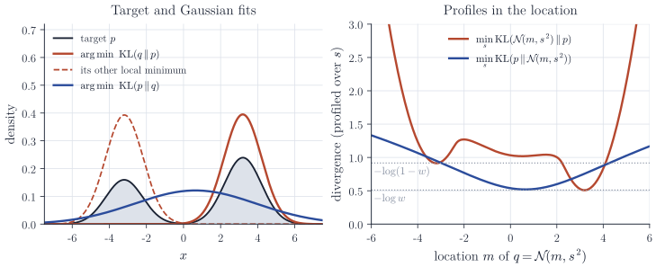
Mixture target with reverse and forward KL Gaussian fits, and both divergences as functions of the location — Figure 1. Target $p_a$ with $w = 0.6$, $a = 3.2$. Left: the global minimizer of $\mathrm{KL}(q\Vert p)$ over Gaussians, its local minimizer at the lighter component, and the moment-matched minimizer of $\mathrm{KL}(p\Vert q)$. Right: both divergences minimized over the scale $s$ for each location $m$; dotted lines mark $-\log w$ and $-\log(1-w)$, the limits from Proposition 2. Expectations under $q$ are computed by the trapezoidal rule on a fine grid.

In Figure 1 the reverse fit is $\mathcal N(3.19, 1.01^2)$ with divergence $0.509$, just below $-\log 0.6 \approx 0.511$, and a second local minimum sits on the lighter component at height $0.914$, close to $-\log 0.4 \approx 0.916$. A third, shallow local minimum is the broad fit $\mathcal N(0.50, 2.84^2)$ with divergence $1.02$. Which local minimum a gradient-based optimizer reaches depends on its initialization, and the lighter component is a perfectly stable answer. The forward profile, in contrast, is unimodal in $m$.

Moderate separation

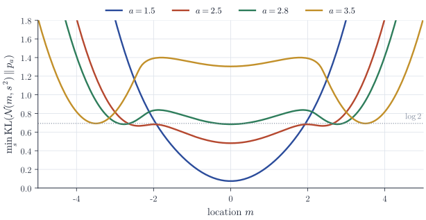
Proposition 2 is asymptotic, and the phrase “mode-seeking” is easy to over-apply. With equal weights the reverse fit is the broad, centred Gaussian whenever the components overlap appreciably; Figure 2 shows the profile $m \mapsto \min_s \mathrm{KL}(\mathcal N(m,s^2)\Vert p_a)$ for several separations. For $a = 1.5$ there is a single minimum at $m = 0$. Around $a = 2.5$ two further local minima appear near $\pm a$ while the centred one remains global; at $a \approx 2.80$ the three minima have equal height, and beyond that the component-centred fits win. The switch is discontinuous: the optimal location jumps from $0$ to roughly $\pm a$ without passing through intermediate values.

Reverse KL profiled over the scale, as a function of the location, for four separations — Figure 2. Equal weights $w = 1/2$. Reverse divergence minimized over $s$, as a function of the location $m$, for separations $a \in \{1.5, 2.5, 2.8, 3.5\}$. The centred minimum rises like a multiple of $a^2$, while the minima near $\pm a$ approach $\log 2$ from below.

Mean-field fits to a correlated Gaussian

The same asymmetry shows up without any multimodality when the family cannot represent dependence. Let $p = \mathcal N(\mu, \Sigma)$ on $\R^d$ with $\Sigma$ positive definite and precision matrix $\Lambda = \Sigma^{-1}$, and let $\mathcal Q_{\mathrm{MF}}$ be the Gaussian product family $q = \bigotimes_{i=1}^d \mathcal N(m_i, v_i)$.

Proposition 3. Over $\mathcal Q_{\mathrm{MF}}$:

$\mathrm{KL}(q\Vert p)$ is uniquely minimized by $m = \mu$ and $v_i = 1/\Lambda_{ii}$;
$\mathrm{KL}(p\Vert q)$ is uniquely minimized by $m = \mu$ and $v_i = \Sigma_{ii}$;
$1/\Lambda_{ii} \le \Sigma_{ii}$ for each $i$, with equality if and only if $\Sigma_{ij} = 0$ for all $j \ne i$.

Proof. For Gaussians $q = \mathcal N(m, V)$ and $p = \mathcal N(\mu, \Sigma)$,

\[\mathrm{KL}(q\Vert p) = \tfrac12 \Bigl[ \tr(\Lambda V) + (m - \mu)^\top \Lambda (m - \mu) - d - \log\det V - \log \det \Lambda \Bigr].\]

(1) With $V = \diag(v_1, \dots, v_d)$, $\tr(\Lambda V) - \log\det V = \sum_i (\Lambda_{ii} v_i - \log v_i)$. Each summand is strictly convex in $v_i > 0$ with minimum at $v_i = 1/\Lambda_{ii}$, and the quadratic term vanishes only at $m = \mu$ because $\Lambda$ is positive definite.

(2) Swapping roles in the same formula, $\mathrm{KL}(p\Vert q) = \tfrac12 \sum_i \bigl[ (\Sigma_{ii} + (\mu_i - m_i)^2)/v_i + \log v_i \bigr] + \text{const}$, and each summand is minimized uniquely at $m_i = \mu_i$, $v_i = \Sigma_{ii}$.

(3) Partition the coordinates into $i$ and the rest, $-i$. The block-inversion formula gives

\[\frac{1}{\Lambda_{ii}} = \Sigma_{ii} - \Sigma_{i,-i} \, \Sigma_{-i,-i}^{-1} \, \Sigma_{-i,i},\]

and the subtracted quadratic form is non-negative, vanishing exactly when $\Sigma_{-i,i} = 0$, since $\Sigma_{-i,-i}^{-1}$ is positive definite.

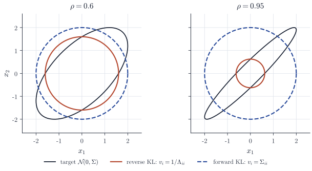
The right-hand side of the block-inversion formula is $\Var(X_i \mid X_{-i})$ for $X \sim p$. So the reverse mean-field fit assigns each coordinate its conditional variance given all other coordinates, while the forward fit assigns the marginal variance. For a bivariate target with unit variances and correlation $\rho$ the two answers are $1 - \rho^2$ and $1$. The volumes compare in the same way: Hadamard’s inequality $\det\Lambda \le \prod_i \Lambda_{ii}$ gives $\prod_i \Lambda_{ii}^{-1} \le \det \Sigma \le \prod_i \Sigma_{ii}$, the second inequality being Hadamard’s inequality for $\Sigma$. The reverse fit is too concentrated, the forward fit too diffuse.

Two-standard-deviation ellipses of a correlated Gaussian and of its reverse and forward mean-field fits — Figure 3. Contours at Mahalanobis radius 2 of a bivariate Gaussian with unit variances and correlation $\rho$, and of its mean-field fits under the reverse divergence (variances $1-\rho^2$) and the forward divergence (variances $1$).

Part 1 remains true when $\mathcal Q_{\mathrm{MF}}$ is enlarged to all product densities $q = \prod_i q_i$. If some factor has infinite variance, the divergence is infinite; this follows from the Donsker–Varadhan inequality $\E_q f \le \mathrm{KL}(q\Vert p) + \log \E_p e^{f}$, valid for measurable $f \ge 0$, applied to $f(x) = \varepsilon \norm{x - \mu}^2$ with $\varepsilon > 0$ small enough that $\E_p e^f < \infty$. Otherwise

\[\mathrm{KL}(q\Vert p) = -\sum_{i} H(q_i) + \tfrac12 \E_q (X - \mu)^\top \Lambda (X - \mu) + \text{const},\]

and by independence of the coordinates under $q$ the expectation depends on $q$ only through the means and variances of the factors. For a given mean and variance the entropy $H(q_i)$ is largest when $q_i$ is Gaussian, so replacing every factor by the Gaussian with the same first two moments never increases the divergence. The underdispersion of mean-field approximations is therefore caused by the divergence together with the factorization; restricting the factors to be Gaussian plays no role.

Remarks

Both examples point in the same direction. Under $\mathrm{KL}(q\Vert p)$ the approximation is judged on the region where $q$ lives, so it is cheap to ignore part of $p$ and expensive to spread into regions where $p$ is small. In Bayesian applications this means that variational posteriors tend to understate uncertainty, and that multimodal posteriors are often represented by a single mode selected by initialization.

Several families of divergences interpolate between the two directions, among them Amari’s $\alpha$-divergences and the Rényi divergences used for variational inference by Li and Turner (Rényi divergence variational inference, 2016). Minka’s technical report Divergence measures and message passing (2005) compares the behaviour of these divergences on examples of the kind above. Expectation propagation minimizes forward divergences locally and accordingly produces mass-covering approximations. For background see Chapter 10 of Bishop, Pattern Recognition and Machine Learning, and Blei, Kucukelbir and McAuliffe, Variational inference: a review for statisticians (JASA, 2017).