Ridge regression as a linear system: augmentation, the dual form and the minimum-norm limit

Ridge regression is usually introduced as a fix for an ill-conditioned matrix $X^\top X$: add $\lambda I$ to the diagonal and invert. Most of what is useful about the estimator follows from that one algebraic move, and the singular value decomposition of the design makes all of it explicit. The linear algebra below covers existence and uniqueness, an augmented least-squares form, a dual form that involves only inner products between observations, the behaviour at the two ends of the regularization path, and an exact formula for leave-one-out residuals.

Throughout, $X \in \R^{n \times p}$ is a fixed design matrix, $y \in \R^n$ a response vector and $\lambda > 0$. No relation between $n$ and $p$ is assumed, and $X$ need not have full rank. The ridge criterion is

\[L_\lambda(\beta) = \lVert y - X\beta\rVert ^2 + \lambda \lVert \beta\rVert ^2, \qquad \beta \in \R^p,\]

with $\lVert \cdot\rVert$ the Euclidean norm. I leave the intercept out; in practice it is either left unpenalized after centering $X$ and $y$, or absorbed into $X$ as a column of ones and penalized like the other coefficients. Everything below applies to the second convention as stated and to the first after centering, with one exception noted at the end.

Existence, uniqueness and the augmented design

Proposition 1. For every $\lambda > 0$ the matrix $X^\top X + \lambda I_p$ is positive definite, and $L_\lambda$ has the unique minimizer

\[\hat\beta_\lambda = (X^\top X + \lambda I_p)^{-1} X^\top y .\]

Proof. For $v \neq 0$, $v^\top (X^\top X + \lambda I_p) v = \lVert Xv\rVert ^2 + \lambda \lVert v\rVert ^2 \ge \lambda \lVert v\rVert ^2 > 0$. Write $A = X^\top X + \lambda I_p$ and $\hat\beta = A^{-1} X^\top y$. Expanding the squares gives $L_\lambda(\beta) = y^\top y - 2\beta^\top X^\top y + \beta^\top A \beta$, and substituting $X^\top y = A\hat\beta$ and completing the square,

\[L_\lambda(\beta) = L_\lambda(\hat\beta) + (\beta - \hat\beta)^\top A (\beta - \hat\beta).\]

The second term is positive unless $\beta = \hat\beta$.

The same criterion is an ordinary least-squares problem with $p$ extra rows. Let

\[\tilde X = \begin{pmatrix} X \\ \sqrt{\lambda}\, I_p \end{pmatrix} \in \R^{(n+p) \times p}, \qquad \tilde y = \begin{pmatrix} y \\ 0 \end{pmatrix} \in \R^{n+p}.\]

Then $\lVert \tilde y - \tilde X \beta\rVert ^2 = \lVert y - X\beta\rVert ^2 + \lVert 0 - \sqrt\lambda\, \beta\rVert ^2 = L_\lambda(\beta)$, and $\tilde X^\top \tilde X = X^\top X + \lambda I_p$. The design $\tilde X$ has full column rank whatever $X$ is, because its lower block does. Each added row is a pseudo-observation recording the value zero for one coefficient, weighted by $\lambda$ relative to a real observation. Two practical consequences follow. Any least-squares routine computes ridge estimates, and a QR factorization of $\tilde X$ does so without ever forming $X^\top X$, whose condition number is the square of that of $X$. The augmented form also reads ridge regression as a Bayesian posterior mode: under $y \mid \beta \sim N(X\beta, \sigma^2 I_n)$ and the prior $\beta \sim N(0, (\sigma^2/\lambda) I_p)$, the negative log posterior is $L_\lambda(\beta)/(2\sigma^2)$ plus a constant.

The estimator in singular coordinates

Let $r = \rank X$ and let $X = U D V^\top$ be a thin singular value decomposition: $U \in \R^{n \times r}$ and $V \in \R^{p \times r}$ have orthonormal columns, and $D = \diag(d_1, \dots, d_r)$ with $d_1 \ge \cdots \ge d_r > 0$. The columns of $V$ span the row space of $X$, and $I_p - VV^\top$ is the orthogonal projector onto its null space.

Proposition 2. For every $\lambda > 0$,

\[\hat\beta_\lambda = \sum_{j=1}^{r} \frac{d_j}{d_j^2 + \lambda}\, (u_j^\top y)\, v_j , \qquad X\hat\beta_\lambda = \sum_{j=1}^r \frac{d_j^2}{d_j^2 + \lambda}\, (u_j^\top y)\, u_j ,\]

where $u_j, v_j$ are the columns of $U, V$. In particular $\hat\beta_\lambda$ lies in the row space of $X$.

Proof. Since $X^\top X = V D^2 V^\top$, we have $X^\top X + \lambda I_p = V(D^2 + \lambda I_r)V^\top + \lambda (I_p - VV^\top)$. The two terms act on orthogonal complementary subspaces, so the inverse is

\[(X^\top X + \lambda I_p)^{-1} = V(D^2 + \lambda I_r)^{-1} V^\top + \lambda^{-1}(I_p - VV^\top),\]

as one checks by multiplying out and using $V^\top V = I_r$. Applying it to $X^\top y = V D U^\top y$ kills the second term, because $(I_p - VV^\top)V = 0$, and leaves $V (D^2 + \lambda I_r)^{-1} D U^\top y$. Multiplying by $X = UDV^\top$ gives the fitted values.

The fitted values are $H_\lambda y$ with the hat matrix

\[H_\lambda = X (X^\top X + \lambda I_p)^{-1} X^\top = U \diag\Bigl(\frac{d_j^2}{d_j^2 + \lambda}\Bigr) U^\top .\]

Unlike the least-squares hat matrix, $H_\lambda$ is symmetric but not idempotent: its nonzero eigenvalues $d_j^2/(d_j^2+\lambda)$ lie strictly between $0$ and $1$. Its trace, $\mathrm{df}(\lambda) = \sum_{j} d_j^2 / (d_j^2 + \lambda)$, decreases from $r$ to $0$ as $\lambda$ increases and is the usual definition of the effective degrees of freedom of the fit. One SVD gives the whole path: after computing $U, D, V$ once, each new value of $\lambda$ costs $O(pr)$ operations.

The dual form

When $p$ is much larger than $n$, inverting a $p \times p$ matrix is wasteful, since $\hat\beta_\lambda$ lives in the row space of $X$, of dimension at most $n$. The identity that moves the computation to $\R^n$ is

\[(X^\top X + \lambda I_p)^{-1} X^\top = X^\top (X X^\top + \lambda I_n)^{-1}.\]

To prove it, note that $X^\top (XX^\top + \lambda I_n) = (X^\top X + \lambda I_p) X^\top$; both sides equal $X^\top X X^\top + \lambda X^\top$. Multiply on the left by $(X^\top X + \lambda I_p)^{-1}$ and on the right by $(XX^\top + \lambda I_n)^{-1}$, both of which exist by Proposition 1 applied to $X$ and to $X^\top$. Hence

\[\hat\beta_\lambda = X^\top \hat\alpha_\lambda, \qquad \hat\alpha_\lambda = (K + \lambda I_n)^{-1} y, \qquad K = X X^\top .\]

The cost is one $n \times n$ solve, and the data enter only through the Gram matrix $K_{ik} = x_i^\top x_k$ of the rows $x_i^\top$ of $X$. The prediction at a new point $x_0$ is $x_0^\top \hat\beta_\lambda = \sum_i \hat\alpha_{\lambda, i}\, x_0^\top x_i$, again a function of inner products only. Replacing $x^\top x'$ by a positive semi-definite kernel $k(x, x')$ gives kernel ridge regression with no further derivation; the representer theorem is the infinite-dimensional version of the statement that $\hat\beta_\lambda$ lies in the span of the observed $x_i$.

The two ends of the path

As $\lambda \to \infty$, every coefficient in Proposition 2 vanishes, and more precisely $\lambda \hat\beta_\lambda = \sum_j \lambda d_j (d_j^2 + \lambda)^{-1} (u_j^\top y) v_j \to \sum_j d_j (u_j^\top y) v_j = X^\top y$. Heavily penalized ridge is a small step from zero in the direction $X^\top y$, which is the negative gradient of $\tfrac12\lVert y - X\beta\rVert ^2$ at $\beta = 0$.

The limit $\lambda \to 0$ is more interesting when $X$ is rank deficient, for example when $p > n$. Least squares then has infinitely many solutions, and ridge regression selects one of them.

Proposition 3. Let $X^{+} = V D^{-1} U^\top$ be the Moore–Penrose pseudoinverse. Among all minimizers of $\lVert y - X\beta\rVert ^2$, the vector $X^+ y$ is the unique one of smallest Euclidean norm, and for every $\lambda > 0$

\[\lVert \hat\beta_\lambda - X^{+} y\rVert \le \frac{\lambda}{d_r^2 + \lambda}\, \lVert X^+ y\rVert \le \frac{\lambda}{d_r^2}\, \lVert X^+ y\rVert .\]

In particular $\hat\beta_\lambda \to X^+ y$ as $\lambda \downarrow 0$.

Proof. The minimizers of $\lVert y - X\beta\rVert ^2$ solve the normal equations $X^\top X \beta = X^\top y$. The vector $X^+ y$ solves them, since $X^\top X X^+ y = V D^2 V^\top V D^{-1} U^\top y = V D U^\top y = X^\top y$, so the solution set is $X^+y + \ker X$ (note $\ker X^\top X = \ker X$). Because $X^+ y$ lies in the range of $V$, which is orthogonal to $\ker X$, Pythagoras gives $\lVert X^+ y + w\rVert ^2 = \lVert X^+ y\rVert ^2 + \lVert w\rVert ^2$ for $w \in \ker X$, minimized only at $w = 0$.

For the bound, Proposition 2 and $X^+ y = \sum_j d_j^{-1}(u_j^\top y) v_j$ give

\[X^+ y - \hat\beta_\lambda = \sum_{j=1}^r \Bigl(\frac{1}{d_j} - \frac{d_j}{d_j^2 + \lambda}\Bigr)(u_j^\top y)\, v_j = \sum_{j=1}^r \frac{\lambda}{d_j^2 + \lambda} \cdot \frac{u_j^\top y}{d_j}\, v_j .\]

The $v_j$ are orthonormal, and each factor $\lambda / (d_j^2 + \lambda)$ is at most $\lambda / (d_r^2 + \lambda)$.

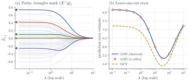
When $r = n < p$ the minimum-norm solution interpolates the data, $X X^+ y = U U^\top y = y$. Ridge regression with a vanishing penalty is therefore the minimum-norm interpolator, the object behind recent analyses of interpolating estimators in overparameterized regression. The bound also shows how fast the limit is reached: $\lambda$ is small, for this purpose, once it is small compared with the smallest nonzero squared singular value $d_r^2$. Panel (a) of Figure 1 shows the paths for a simulated design with $n = 30$ and $p = 60$, for which $d_r^2 \approx 3.7$; for $\lambda$ well below this value the paths are flat at the coordinates of $X^+ y$.

Ridge coefficient paths flattening at the minimum-norm solution for small lambda, and leave-one-out error curves computed by the shortcut formula and by refitting — Figure 1. Simulated design with $n = 30$, $p = 60$, AR(1) correlated covariates ($\rho = 0.6$), five nonzero coefficients and noise standard deviation $2$. (a) Ridge paths; the five coordinates with nonzero true coefficients are coloured, the rest are grey. As $\lambda \downarrow 0$ the paths settle at the minimum-norm least-squares solution $X^{+}y$ (triangles). (b) Leave-one-out error from the closed form of Proposition 4 (line) and from $n$ separate refits (circles), with generalized cross-validation for comparison.

Leave-one-out residuals without refitting

Choosing $\lambda$ by leave-one-out cross-validation appears to need $n$ refits per value of $\lambda$. Because the estimator is linear in $y$ and the left-out row enters $X^\top X$ as a rank-one term, the refits can be avoided. Write $x_i^\top$ for the $i$th row of $X$, $\hat y_i = x_i^\top \hat\beta_\lambda$, $h_{ii}$ for the $i$th diagonal entry of $H_\lambda$, and $\hat\beta_\lambda^{(-i)}$ for the ridge estimate computed without observation $i$ (with the same $\lambda$).

Proposition 4. For every $\lambda > 0$ and every $i$, $h_{ii} < 1$ and

\[y_i - x_i^\top \hat\beta_\lambda^{(-i)} = \frac{y_i - \hat y_i}{1 - h_{ii}} .\]

Proof. From the spectral form of $H_\lambda$, $h_{ii} = \sum_j U_{ij}^2\, d_j^2/(d_j^2 + \lambda)$. If the $i$th row of $U$ is zero, $h_{ii} = 0$; otherwise $h_{ii} < \sum_j U_{ij}^2 \le 1$, the last inequality because $UU^\top$ is an orthogonal projector and its diagonal entries are at most one.

Let $A = X^\top X + \lambda I_p$, so that $h_{ii} = x_i^\top A^{-1} x_i$. Deleting row $i$ replaces $A$ by $A - x_i x_i^\top$ and $X^\top y$ by $X^\top y - y_i x_i$. Since $1 - h_{ii} \neq 0$, the Sherman–Morrison formula applies:

\[(A - x_i x_i^\top)^{-1} = A^{-1} + \frac{A^{-1} x_i x_i^\top A^{-1}}{1 - h_{ii}} .\]

Multiplying on the left by $x_i^\top$ gives $x_i^\top (A - x_i x_i^\top)^{-1} = x_i^\top A^{-1} / (1 - h_{ii})$. Hence

\[x_i^\top \hat\beta_\lambda^{(-i)} = \frac{x_i^\top A^{-1}(X^\top y - y_i x_i)}{1 - h_{ii}} = \frac{\hat y_i - h_{ii} y_i}{1 - h_{ii}},\]

and subtracting from $y_i$ gives the claim.

The leave-one-out estimate of prediction error is therefore

\[\mathrm{CV}(\lambda) = \frac1n \sum_{i=1}^n \Bigl(\frac{y_i - \hat y_i}{1 - h_{ii}}\Bigr)^2 ,\]

and with the SVD in hand both $\hat y$ and the $h_{ii}$ are available for every $\lambda$ at negligible cost. Panel (b) of Figure 1 checks the formula against brute-force refitting. Generalized cross-validation, proposed for ridge regression by Golub, Heath and Wahba (Technometrics, 1979), replaces every $h_{ii}$ by their average $\mathrm{df}(\lambda)/n$; this makes the criterion invariant under orthogonal transformations of the response space, at the price of ignoring which observations have high leverage.

The second half of the proof uses only that $A$ is the sum of $X^\top X$ and a fixed matrix, and that $A$ and $A - x_i x_i^\top$ are invertible; the latter already forces $h_{ii} \neq 1$, because $\det(A - x_i x_i^\top) = \det(A)\,(1 - h_{ii})$ by the matrix determinant lemma. The identity therefore holds verbatim for generalized ridge penalties $\lambda\, \beta^\top \Omega \beta$ with $\Omega$ positive semi-definite, including the case of an unpenalized intercept column, provided $X^\top X + \lambda\Omega$ and every $X_{(-i)}^\top X_{(-i)} + \lambda \Omega$ are invertible, where $X_{(-i)}$ is $X$ with row $i$ deleted. It fails when $y$ and $X$ are centered with all $n$ observations before fitting, because the left-out point then influences the centering; this is one reason to keep the intercept as a column of $X$ when cross-validating.

Remarks

The material here is standard and spread across Hoerl and Kennard’s original papers in Technometrics (1970), Chapter 3 of Hastie, Tibshirani and Friedman, The Elements of Statistical Learning, and Golub and Van Loan, Matrix Computations, for the SVD and the numerical points. The augmented-design trick is the regression form of Tikhonov regularization, and the dual form is the starting point for Gaussian process regression, where $\hat\alpha_\lambda$ reappears with $\lambda$ equal to the noise variance.