Where ridge regression shrinks: principal directions, bias–variance and a guaranteed improvement over least squares

The phrase “ridge regression shrinks the coefficients towards zero” is true of the coefficient vector as a whole and misleading about its coordinates. The shrinkage happens along the principal axes of the design, by an amount that depends on how much the design varies in each direction. Seen in those coordinates, the bias–variance trade-off is explicit, and the classical result of Hoerl and Kennard, that some amount of ridge penalty always beats least squares in mean squared error, has a two-line proof.

Setting

Let $y = X\beta + \varepsilon$ with a fixed design $X \in \R^{n \times p}$ of full column rank $p$ (so $n \ge p$), $\E \varepsilon = 0$ and $\Cov(\varepsilon) = \sigma^2 I_n$. No distributional assumption beyond the first two moments is needed. For $\lambda \ge 0$ the ridge estimator is

\[\hat\beta_\lambda = (X^\top X + \lambda I_p)^{-1} X^\top y ,\]

and $\hat\beta_0$ is the least-squares estimator $\hat\beta^{\mathrm{OLS}}$. Write the singular value decomposition $X = UDV^\top$ with $U \in \R^{n \times p}$ and $V \in \R^{p \times p}$ having orthonormal columns and $D = \diag(d_1, \dots, d_p)$, $d_1 \ge \cdots \ge d_p > 0$. The columns $v_j$ of $V$ are the principal axes of the design: $d_j^2 = \lVert Xv_j\rVert^2$ measures the spread of the data in direction $v_j$. Coordinates in this basis are denoted

\[\alpha = V^\top \beta, \qquad \hat a = V^\top \hat\beta^{\mathrm{OLS}}, \qquad \hat a_j = \frac{u_j^\top y}{d_j}.\]

Since $V$ is orthogonal, $\lVert \hat\beta - \beta\rVert = \lVert V^\top\hat\beta - \alpha\rVert$ for any estimator, so mean squared errors can be computed in these coordinates.

Shrinkage factors

Substituting the decomposition, $X^\top X + \lambda I_p = V(D^2 + \lambda I_p)V^\top$ and $X^\top y = VDU^\top y$, so

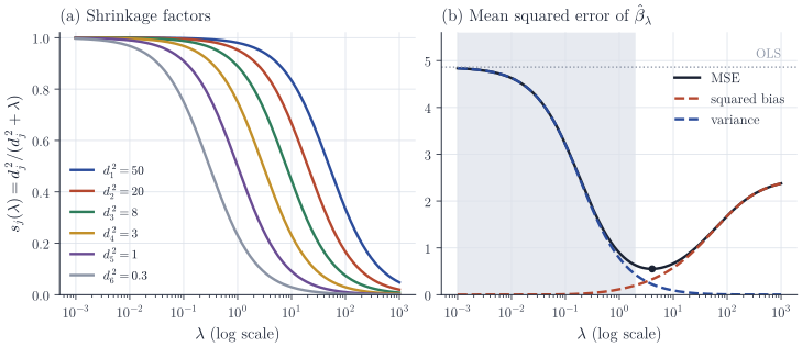
\[V^\top \hat\beta_\lambda = (D^2 + \lambda I_p)^{-1} D U^\top y, \qquad\text{that is,}\qquad (V^\top\hat\beta_\lambda)_j = s_j(\lambda)\, \hat a_j, \quad s_j(\lambda) = \frac{d_j^2}{d_j^2 + \lambda}.\]

Ridge regression takes the least-squares coefficient along each principal axis and multiplies it by $s_j(\lambda) \in (0, 1]$. The factor is close to one when $d_j^2 \gg \lambda$ and close to zero when $d_j^2 \ll \lambda$, so the penalty acts mostly on directions in which the design has little spread, which are exactly the directions in which $\hat a_j$ is noisy: $\Var(\hat a_j) = \sigma^2/d_j^2$. Panel (a) of Figure 2 below shows the factors for six singular values. When the design is orthonormal, $X^\top X = I_p$, all factors equal $1/(1+\lambda)$ and ridge is uniform proportional shrinkage of every coefficient.

In the original coordinates the picture is different. Take two standardized covariates with correlation $0.9$, so that $X^\top X$ has eigenvectors $v_1 \propto (1, 1)$ and $v_2 \propto (1, -1)$ with eigenvalues $1.9$ and $0.1$, and suppose $\hat\beta^{\mathrm{OLS}} = (2, -0.3)$. The component along $v_2$ is already halved at $\lambda = 0.1$, the component along $v_1$ only at $\lambda = 1.9$, and the path bends toward the $v_1$ axis. The second coefficient changes sign and, for a range of $\lambda$, exceeds its least-squares value in absolute value (Figure 1).

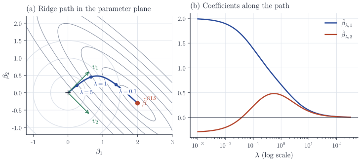
Ridge path in the plane of two coefficients, bending towards the first principal axis, and the two coefficients as functions of lambda — Figure 1. Two covariates with $X^\top X = \begin{pmatrix} 1 & 0.9 \\ 0.9 & 1\end{pmatrix}$ and $\hat\beta^{\mathrm{OLS}} = (2, -0.3)$. (a) Contours of the residual sum of squares (grey ellipses), circles of constant $\lVert\beta\rVert$, and the ridge path from $\hat\beta^{\mathrm{OLS}}$ to the origin. Each point on the path is where a circle touches a contour. (b) The second coefficient changes sign and grows before both coefficients decay.

What does hold is monotonicity of the whole vector. The norm $\lVert \hat\beta_\lambda\rVert^2 = \sum_j s_j(\lambda)^2 \hat a_j^2$ is strictly decreasing in $\lambda$ whenever $\hat\beta^{\mathrm{OLS}} \neq 0$, and the residual sum of squares $\lVert y - X\hat\beta_\lambda\rVert^2$ is nondecreasing. Moreover $\hat\beta_\lambda$ minimizes the residual sum of squares over the ball $\{\beta : \lVert \beta\rVert \le \lVert \hat\beta_\lambda\rVert\}$: if some $\beta$ in that ball had a smaller residual sum of squares, it would also have a smaller value of $\lVert y - X\beta\rVert^2 + \lambda\lVert\beta\rVert^2$, contradicting optimality of $\hat\beta_\lambda$. This is the tangency in panel (a) of Figure 1, and it is the constrained formulation of ridge regression with a data-dependent radius.

Bias, variance and mean squared error

Proposition 1. For every $\lambda \ge 0$,

\[\E \hat\beta_\lambda = V \diag\bigl(s_j(\lambda)\bigr) V^\top \beta, \qquad \Cov(\hat\beta_\lambda) = \sigma^2\, V \diag\Bigl(\frac{d_j^2}{(d_j^2 + \lambda)^2}\Bigr) V^\top ,\]

and

\[\mathrm{MSE}(\lambda) := \E \lVert \hat\beta_\lambda - \beta\rVert^2 = \sum_{j=1}^p \underbrace{\frac{\lambda^2 \alpha_j^2}{(d_j^2 + \lambda)^2}}_{\text{squared bias}} + \underbrace{\frac{\sigma^2 d_j^2}{(d_j^2+\lambda)^2}}_{\text{variance}} .\]

Proof. Let $w = U^\top y$. Since $U^\top X\beta = DV^\top\beta = D\alpha$, we have $\E w = D\alpha$ and $\Cov(w) = \sigma^2 U^\top U = \sigma^2 I_p$. The coordinates $(V^\top\hat\beta_\lambda)_j = d_j w_j / (d_j^2 + \lambda)$ are therefore uncorrelated, with mean $s_j(\lambda)\alpha_j$ and variance $\sigma^2 d_j^2/(d_j^2+\lambda)^2$. Transforming back with $V$ gives the first two claims. For the third, $\E\lVert \hat\beta_\lambda - \beta\rVert^2$ is the sum over $j$ of the squared bias $(1 - s_j(\lambda))^2 \alpha_j^2$ and the variance of the $j$th coordinate, and $1 - s_j(\lambda) = \lambda/(d_j^2 + \lambda)$.

At $\lambda = 0$ the bias vanishes and $\mathrm{MSE}(0) = \sigma^2 \sum_j d_j^{-2}$, which is large as soon as one singular value is small, regardless of $\beta$. The variance terms decrease in $\lambda$ and the bias terms increase from zero. The covariance comparison is in fact uniform: since $d_j^2/(d_j^2+\lambda)^2 < 1/d_j^2$ for $\lambda > 0$, the matrix $\Cov(\hat\beta^{\mathrm{OLS}}) - \Cov(\hat\beta_\lambda)$ is positive definite, so every linear combination $c^\top \hat\beta_\lambda$ has strictly smaller variance than $c^\top\hat\beta^{\mathrm{OLS}}$.

A guaranteed improvement

Hoerl and Kennard (Technometrics, 1970) showed that there is always a $\lambda > 0$ with $\mathrm{MSE}(\lambda) < \mathrm{MSE}(0)$. The decomposition in Proposition 1 gives an explicit range, by comparing the summands one at a time.

Theorem 2. Let $\alpha_{\max}^2 = \max_j \alpha_j^2$. If $\alpha_{\max} = 0$ then $\mathrm{MSE}(\lambda) < \mathrm{MSE}(0)$ for all $\lambda > 0$. Otherwise this holds for all $0 < \lambda < 2\sigma^2/\alpha_{\max}^2$, and in particular whenever $0 < \lambda < 2\sigma^2/\lVert\beta\rVert^2$.

Proof. Fix $j$ and $\lambda > 0$. The $j$th summand of $\mathrm{MSE}(\lambda)$ is smaller than its value $\sigma^2/d_j^2$ at $\lambda = 0$ if and only if

\[d_j^2(\lambda^2\alpha_j^2 + \sigma^2 d_j^2) < \sigma^2 (d_j^2 + \lambda)^2 \iff d_j^2 \lambda^2 \alpha_j^2 < \sigma^2(2 d_j^2 \lambda + \lambda^2) \iff \lambda\, d_j^2 \alpha_j^2 < \sigma^2 (2 d_j^2 + \lambda),\]

after multiplying out, cancelling $\sigma^2 d_j^4$ and dividing by $\lambda > 0$. If $\lambda \alpha_j^2 < 2\sigma^2$, the left-hand side is less than $2\sigma^2 d_j^2$, which is at most the right-hand side. Hence every summand strictly decreases when $\lambda < 2\sigma^2/\alpha_{\max}^2$ (or for every $\lambda > 0$ if all $\alpha_j = 0$). The last statement follows from $\alpha_{\max}^2 \le \lVert\alpha\rVert^2 = \lVert\beta\rVert^2$.

The guaranteed range is governed by a signal-to-noise ratio and does not depend on the design. The design determines how large the gain is: $\mathrm{MSE}(0)$ blows up as $d_p \to 0$, while the ridge risk stays bounded by $\lVert\beta\rVert^2 + \sigma^2\sum_j d_j^2/(d_j^2+\lambda)^2 \le \lVert\beta\rVert^2 + p\sigma^2/(4\lambda)$, using $d^2/(d^2+\lambda)^2 \le 1/(4\lambda)$.

The derivative of the $j$th summand is

\[\frac{\dd}{\dd\lambda}\, \frac{\lambda^2\alpha_j^2 + \sigma^2 d_j^2}{(d_j^2+\lambda)^2} = \frac{2 d_j^2 (\lambda \alpha_j^2 - \sigma^2)}{(d_j^2 + \lambda)^3},\]

so the $j$th summand alone is minimized at $\lambda_j^\star = \sigma^2/\alpha_j^2$. With a single penalty, $\mathrm{MSE}'(\lambda)$ is negative for $\lambda < \sigma^2/\alpha_{\max}^2$ and, if $\alpha_{\min}^2 = \min_j \alpha_j^2 > 0$, positive for $\lambda > \sigma^2/\alpha_{\min}^2$; every minimizer of $\mathrm{MSE}$ over $[0, \infty)$ therefore lies between these two values. Allowing a separate penalty $\lambda_j$ along each principal axis (generalized ridge regression) attains every $\lambda_j^\star$ simultaneously. The quantity $\sigma^2/\alpha_j^2$ also has a Bayesian reading: if the errors are Gaussian and the $\alpha_j$ are independent $N(0, \tau^2)$ a priori (equivalently $\beta \sim N(0, \tau^2 I_p)$), the posterior mean is $\hat\beta_\lambda$ with $\lambda = \sigma^2/\tau^2$, and $\tau^2$ plays the role of a typical $\alpha_j^2$.

Shrinkage factors for six singular values, and the mean squared error of ridge regression decomposed into squared bias and variance — Figure 2. A design with squared singular values $d_j^2 = 50, 20, 8, 3, 1, 0.3$, coefficients $\alpha = (1, -0.8, 0.6, 0.5, -0.4, 0.3)$ in the principal basis, and $\sigma^2 = 1$. (a) Shrinkage factors $s_j(\lambda)$. (b) Mean squared error and its two parts. Least squares has risk $\sigma^2\sum_j d_j^{-2} \approx 4.86$, most of it from the smallest singular value. The shaded interval $(0, 2\sigma^2/\alpha_{\max}^2)$ is where Theorem 2 guarantees an improvement; the minimum, $0.55$ at $\lambda \approx 4.1$, lies between $\sigma^2/\alpha_{\max}^2 = 1$ and $\sigma^2/\alpha_{\min}^2 \approx 11.1$.

What the theorem does not say

Theorem 2 is a statement about deterministic $\lambda$, and the admissible range depends on the unknown ratio $\sigma^2/\alpha_{\max}^2$. An estimator that chooses $\lambda$ from the data, by cross-validation or by plugging estimates of $\sigma^2$ and $\alpha$ into $\lambda_j^\star$, is a nonlinear function of $y$ and does not inherit the guarantee automatically. Whether such an adaptive estimator dominates least squares is a separate question, closely related to Stein’s phenomenon, and the answer depends on the dimension and the spread of the singular values.

The criterion also matters. The prediction risk $\E\lVert X\hat\beta_\lambda - X\beta\rVert^2 = \sum_j d_j^2 \bigl[(1 - s_j)^2\alpha_j^2 + s_j^2\sigma^2/d_j^2\bigr]$ weights direction $j$ by $d_j^2$, so low-variance directions, where ridge does most of its work, count for less. Repeating the argument of Theorem 2 summand by summand gives the same sufficient condition $\lambda < 2\sigma^2/\alpha_{\max}^2$ for improving on least squares in prediction, since each summand is the corresponding summand of $\mathrm{MSE}(\lambda)$ multiplied by $d_j^2$.

Finally, the shrinkage factors make the comparison with principal component regression immediate. Principal component regression on the first $k$ components replaces $s_j(\lambda)$ by the indicator of $j \le k$: it keeps high-variance directions untouched and discards the rest. Ridge regression is the smooth version, which never discards a direction completely and never leaves one completely untouched. The standard reference for both is Chapter 3 of Hastie, Tibshirani and Friedman, The Elements of Statistical Learning; the algebra of the ridge estimator itself is treated in a companion note.