Schur complements: block elimination, Gaussian conditioning and partial correlation
Eliminate the first block of unknowns from a linear system with a \(2 \times 2\) block matrix, and the system that remains for the second block has the coefficient matrix \(D - CA^{-1}B\). This matrix, the Schur complement, appears in statistics whenever variables are split into two groups: it is the covariance of the second group after the linear effect of the first has been removed, and for Gaussian vectors it is the conditional covariance. The algebra is developed first; the statistical facts then follow from it with little extra work.
Throughout,
\[M = \begin{pmatrix} A & B \\ C & D \end{pmatrix}, \qquad A \in \R^{k \times k},\ D \in \R^{m \times m},\]and when \(A\) is invertible the Schur complement of \(A\) in \(M\) is \(M/A = D - CA^{-1}B\). Symmetrically, when \(D\) is invertible, \(M/D = A - BD^{-1}C\).
Block elimination
Proposition 1. Suppose \(A\) is invertible and write \(S = M/A\). Then
\[M = \begin{pmatrix} I_k & 0 \\ CA^{-1} & I_m \end{pmatrix} \begin{pmatrix} A & 0 \\ 0 & S \end{pmatrix} \begin{pmatrix} I_k & A^{-1}B \\ 0 & I_m \end{pmatrix}.\]Consequently \(\det M = \det A \cdot \det S\), and \(M\) is invertible if and only if \(S\) is, in which case
\[M^{-1} = \begin{pmatrix} A^{-1} + A^{-1}BS^{-1}CA^{-1} & -A^{-1}BS^{-1} \\ -S^{-1}CA^{-1} & S^{-1} \end{pmatrix}.\]Proof. Multiplying the three factors gives \(\begin{pmatrix} A & B \\ C & CA^{-1}B + S\end{pmatrix} = M\). The outer factors are block unit triangular, so they have determinant one and inverses obtained by negating the off-diagonal block. The determinant formula follows, and so does invertibility. Inverting the product in reverse order,
\[M^{-1} = \begin{pmatrix} I_k & -A^{-1}B \\ 0 & I_m \end{pmatrix} \begin{pmatrix} A^{-1} & 0 \\ 0 & S^{-1} \end{pmatrix} \begin{pmatrix} I_k & 0 \\ -CA^{-1} & I_m \end{pmatrix},\]and multiplying out gives the displayed blocks.
In particular, the bottom-right block of the inverse is the inverse of the Schur complement, \((M^{-1})_{22} = (M/A)^{-1}\). Eliminating from the other side, when \(D\) is invertible, gives in the same way \((M^{-1})_{11} = (M/D)^{-1}\) and \((M^{-1})_{12} = -(M/D)^{-1}BD^{-1}\).
Computing the top-left block of \(M^{-1}\) both ways, when \(A\), \(D\) and \(M\) are all invertible, yields
\[(A - BD^{-1}C)^{-1} = A^{-1} + A^{-1}B\,(D - CA^{-1}B)^{-1} CA^{-1}.\]Substituting \(B = U\), \(C = V\) and \(D = -G^{-1}\) turns this into the Woodbury identity
\[(A + UGV)^{-1} = A^{-1} - A^{-1}U\,(G^{-1} + VA^{-1}U)^{-1} VA^{-1},\]valid whenever \(A\), \(G\) and \(G^{-1} + VA^{-1}U\) are invertible. Its main use in statistics is with covariance matrices of the form \(\sigma^2 I_n + WW^\top\) with \(W \in \R^{n \times q}\) and \(q \ll n\), as in factor analysis and Gaussian processes with low-rank structure: the identity replaces an \(n \times n\) inverse by a \(q \times q\) one.
Positive definiteness and a variational form
For symmetric \(M\) with \(C = B^\top\) and \(A \succ 0\), the factorization of Proposition 1 is a congruence, \(M = L \diag(A, S) L^\top\) with \(L\) invertible. Expanding the quadratic form makes this concrete.
Proposition 2. Let \(M\) be symmetric with \(A \succ 0\) and \(S = D - B^\top A^{-1} B\). For all \(x_1 \in \R^k\) and \(x_2 \in \R^m\),
\[\begin{pmatrix} x_1 \\ x_2 \end{pmatrix}^{\!\top} M \begin{pmatrix} x_1 \\ x_2 \end{pmatrix} = (x_1 + A^{-1}Bx_2)^\top A\, (x_1 + A^{-1}Bx_2) + x_2^\top S x_2 .\]Hence \(M \succ 0\) if and only if \(S \succ 0\), \(M \succeq 0\) if and only if \(S \succeq 0\), and
\[x_2^\top S\, x_2 = \min_{x_1 \in \R^k} \begin{pmatrix} x_1 \\ x_2 \end{pmatrix}^{\!\top} M \begin{pmatrix} x_1 \\ x_2 \end{pmatrix},\]the minimum being attained only at \(x_1 = -A^{-1}Bx_2\).
Proof. Expand the right-hand side: the cross terms are \(2x_1^\top B x_2\) and the \(x_2\) terms are \(x_2^\top B^\top A^{-1} B x_2 + x_2^\top D x_2 - x_2^\top B^\top A^{-1}B x_2\). The first summand is nonnegative and vanishes only when \(x_1 = -A^{-1}Bx_2\), which gives the minimum. If \(S \succ 0\) the form is positive unless \(x_2 = 0\) and \(x_1 = 0\); conversely, choosing \(x_1 = -A^{-1}Bx_2\) shows the form equals \(x_2^\top S x_2\), so positivity of \(M\) forces positivity of \(S\). The semi-definite case is identical.
The variational form says that the Schur complement is what is left of a quadratic form after the first block of variables has been optimized out. Applied to a centred Gaussian density proportional to \(\exp(-\tfrac12 x^\top \Omega x)\), with precision matrix \(\Omega \succ 0\), the decomposition shows that integrating out \(x_1\) leaves \(\exp(-\tfrac12 x_2^\top (\Omega/\Omega_{11}) x_2)\) times a constant, because the integral of the first summand’s exponential over \(x_1\) does not depend on \(x_2\). The marginal precision of \(X_2\) is therefore \(\Omega/\Omega_{11}\). The next section shows the dual statement, that the conditional covariance of \(X_1\) is a Schur complement of the covariance.
Conditioning a Gaussian vector
Theorem 3. Let \(X = (X_1, X_2) \sim N_{k+m}(\mu, \Sigma)\) with blocks \(\mu_i\) and \(\Sigma_{ij}\), and assume \(\Sigma_{22} \succ 0\). A version of the conditional distribution of \(X_1\) given \(X_2 = x_2\) is
\[N_k\bigl(\mu_1 + \Sigma_{12}\Sigma_{22}^{-1}(x_2 - \mu_2),\ \Sigma/\Sigma_{22}\bigr), \qquad \Sigma/\Sigma_{22} = \Sigma_{11} - \Sigma_{12}\Sigma_{22}^{-1}\Sigma_{21}.\]Proof. Let \(K = \Sigma_{12}\Sigma_{22}^{-1}\) and \(Z = X_1 - KX_2\). The pair \((Z, X_2)\) is a linear transformation of \(X\), hence jointly Gaussian, and
\[\Cov(Z, X_2) = \Sigma_{12} - K\Sigma_{22} = 0 .\]Uncorrelated jointly Gaussian vectors are independent, because the joint characteristic function factorizes. Moreover \(\E Z = \mu_1 - K\mu_2\) and \(\Cov(Z) = \Sigma_{11} - K\Sigma_{21} - \Sigma_{12}K^\top + K\Sigma_{22}K^\top = \Sigma_{11} - \Sigma_{12}\Sigma_{22}^{-1}\Sigma_{21}\). Since \(X_1 = Z + KX_2\) with \(Z\) independent of \(X_2\), for every bounded measurable \(h\) we have \(\E[h(X_1) \mid X_2] = g(X_2)\) almost surely, where \(g(x_2) = \E\, h(Z + Kx_2)\) (Fubini’s theorem applied to the product law of \((Z, X_2)\)). So the conditional law given \(X_2 = x_2\) is the law of \(Z + Kx_2\), which is the stated normal distribution.
The proof does not need \(\Sigma\) or \(\Sigma_{11}\) to be invertible, and it avoids dividing densities. Two features of the result are specific to the Gaussian family and are visible in Figure 1: the conditional mean is linear in \(x_2\), and the conditional covariance does not depend on \(x_2\) at all. Since \(\Sigma/\Sigma_{22} \preceq \Sigma_{11}\), conditioning never increases uncertainty in the Loewner order.
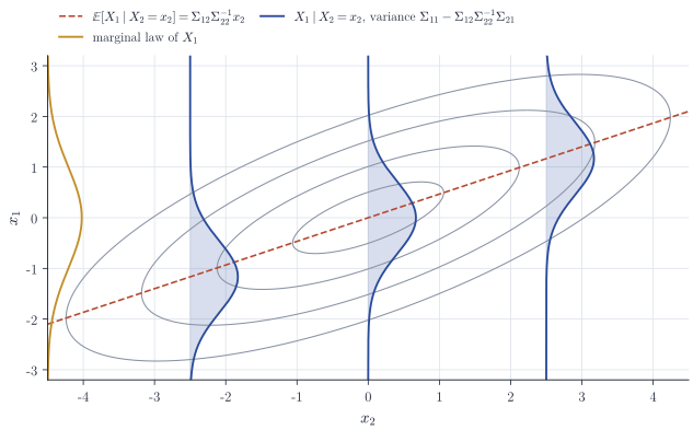
Without the Gaussian assumption half of the statement survives. For any random vector with finite second moments and \(\Sigma_{22} \succ 0\), the computation of \(\Cov(Z, X_2)\) and \(\Cov(Z)\) in the proof is unchanged: \(\mu_1 + K(X_2 - \mu_2)\) is the best linear predictor of \(X_1\) from \(X_2\) in mean square, and \(\Sigma/\Sigma_{22}\) is the covariance of its prediction error. What is lost is the independence of \(Z\) and \(X_2\), and with it the interpretation as a conditional covariance.
Precision matrices and partial correlation
Assume now \(\Sigma \succ 0\) and let \(\Omega = \Sigma^{-1}\) be the precision matrix. By Proposition 1 with the roles of the blocks exchanged, applied to \(\Sigma\), the top-left block of \(\Omega\) is \((\Sigma/\Sigma_{22})^{-1}\). Hence
\[\Cov(X_1 \mid X_2) = (\Omega_{11})^{-1}, \qquad \E[X_1 \mid X_2] = \mu_1 - \Omega_{11}^{-1}\Omega_{12}(X_2 - \mu_2),\]the second identity because the off-diagonal block of \(\Omega\) is \(\Omega_{12} = -(\Sigma/\Sigma_{22})^{-1}\Sigma_{12}\Sigma_{22}^{-1} = -\Omega_{11}\Sigma_{12}\Sigma_{22}^{-1}\), again by Proposition 1 with the roles of the two diagonal blocks exchanged. Conditional quantities are read directly from the precision matrix, with no inversion of \(\Sigma_{22}\).
Take \(X_1 = (X_i, X_j)\) to be two coordinates and \(X_2 = X_R\) the remaining ones. The partial correlation \(\rho_{ij \cdot R}\) is the correlation of \(X_i\) and \(X_j\) under their conditional law given \(X_R\), equivalently the correlation of their residuals after linear regression on \(X_R\).
Corollary 4. If \(X \sim N_p(\mu, \Sigma)\) with \(\Sigma \succ 0\) and \(\Omega = \Sigma^{-1} = (\omega_{ab})\), then for \(i \neq j\)
\[\rho_{ij\cdot R} = -\frac{\omega_{ij}}{\sqrt{\omega_{ii}\,\omega_{jj}}},\]and \(X_i\) and \(X_j\) are conditionally independent given \(X_R\) if and only if \(\omega_{ij} = 0\).
Proof. After permuting coordinates, which permutes rows and columns of \(\Sigma\) and \(\Omega\) consistently, the conditional covariance of \((X_i, X_j)\) given \(X_R\) is the inverse of the \(2 \times 2\) block
\[\begin{pmatrix} \omega_{ii} & \omega_{ij} \\ \omega_{ij} & \omega_{jj} \end{pmatrix}^{-1} = \frac{1}{\omega_{ii}\omega_{jj} - \omega_{ij}^2}\begin{pmatrix} \omega_{jj} & -\omega_{ij} \\ -\omega_{ij} & \omega_{ii} \end{pmatrix},\]whose correlation is the stated ratio. By Theorem 3 the conditional law is bivariate normal, so its coordinates are independent exactly when this correlation is zero.
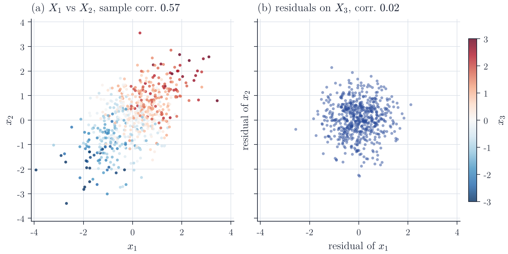
Marginal and partial correlation can be very different. In Figure 2 three variables form a chain, \(X_1\) and \(X_2\) each depending on \(X_3\) and \(\omega_{12} = 0\). The marginal correlation of \(X_1\) and \(X_2\), read off from \(\Sigma = \Omega^{-1}\) (both variances equal \(8/7\), the covariance is \(9/14\)), is \(9/16 \approx 0.56\), all of it transmitted through \(X_3\); the residuals after regressing on \(X_3\) are uncorrelated. The graph whose edges are the nonzero off-diagonal entries of \(\Omega\) is the Gaussian graphical model of \(X\), and estimating a sparse precision matrix, for instance by the graphical lasso, is a way of estimating this conditional independence structure.
Remarks
The same computation explains several standard facts of linear regression. In the regression of \(y\) on a design \((X_1, X_2)\), the block of \((X^\top X)^{-1}\) belonging to \(X_2\) is the inverse of \(X_2^\top X_2 - X_2^\top X_1(X_1^\top X_1)^{-1}X_1^\top X_2 = X_2^\top (I - P_1) X_2\), a Schur complement, where \(P_1\) projects onto the columns of \(X_1\). This is the matrix form of the Frisch–Waugh–Lovell theorem: the coefficients of \(X_2\) are those obtained after residualizing on \(X_1\), and their sampling variance is inflated when \(X_2\) is well predicted by \(X_1\). For a broader survey of Schur complements in matrix analysis, see Zhang (ed.), The Schur Complement and Its Applications; the Gaussian results are in Anderson, An Introduction to Multivariate Statistical Analysis, and Gaussian graphical models are treated in Lauritzen, Graphical Models.