Differentiating an expectation through its density: the score-function gradient estimator

Many objectives in statistics and machine learning are expectations under a distribution that depends on the parameter being optimized:

\[L(\theta) = \E_{\theta} f(X) = \int f(x)\, p_\theta(x)\, \mu(\dd x).\]

The evidence lower bound in variational inference is of this form, with $\theta$ the variational parameters; so is the expected return of a stochastic policy in reinforcement learning, and the price of a financial derivative viewed as a function of a model parameter. Stochastic gradient methods need unbiased estimates of $\nabla L(\theta)$. When $f$ is not differentiable, is available only as a black box, or $X$ is discrete, the gradient cannot be moved onto $f$. It can be moved onto the density instead, by the elementary identity

\[\nabla_\theta p_\theta(x) = p_\theta(x)\, \nabla_\theta \log p_\theta(x) \qquad \text{whenever } p_\theta(x) > 0,\]

which is the chain rule applied to $\log p_\theta(x)$. Under conditions that permit differentiation under the integral sign,

\[\nabla L(\theta) = \int f(x)\, \nabla_\theta p_\theta(x)\, \mu(\dd x) = \E_\theta\bigl[f(X)\, s_\theta(X)\bigr], \qquad s_\theta(x) = \nabla_\theta \log p_\theta(x),\]

and the right-hand side is estimated by $n^{-1}\sum_{j} f(X_j) s_\theta(X_j)$ with $X_j \sim p_\theta$ independent. The function $s_\theta$ is the score of the model, familiar from likelihood theory; here it is evaluated at simulated draws, not at data. The estimator goes by several names: the likelihood-ratio method in the simulation literature, REINFORCE in reinforcement learning, and the log-derivative trick in machine learning.

When the identity holds

Two things must be checked: that $L$ is differentiable with derivative obtained by differentiating inside the integral, and that the points where $p_\theta(x) = 0$ do not contribute.

Theorem 1. Let $\Theta \subseteq \R^d$ be open, $\mu$ a $\sigma$-finite measure on $\mathcal X$, $\{p_\theta : \theta \in \Theta\}$ probability densities with respect to $\mu$, and $f$ measurable. Let $B \subseteq \Theta$ be an open ball, and assume:

for $\mu$-almost every $x$, the map $\theta \mapsto p_\theta(x)$ is continuously differentiable on $B$;
there is a $\mu$-integrable function $h$ with $\abs{f(x)} \sup_{\theta \in B} \norm{\nabla_\theta p_\theta(x)} \le h(x)$ for $\mu$-almost every $x$;
$\E_\theta \abs{f(X)} < \infty$ for $\theta \in B$.

Then $L$ is continuously differentiable on $B$ and $\nabla L(\theta) = \E_\theta[f(X)\, s_\theta(X)]$ for every $\theta \in B$, where $s_\theta(x)$ is defined on $\{p_\theta(x) > 0\}$.

Proof. Fix $\theta \in B$, a unit vector $e$ and $t \ne 0$ small enough that $\theta + te \in B$. For almost every $x$, the mean value theorem applied to $u \mapsto p_{\theta + ue}(x)$ on the segment between $0$ and $t$ gives a point $\theta'$ on that segment, hence in $B$, with

\[\frac{p_{\theta + te}(x) - p_\theta(x)}{t} = e^\top \nabla p_{\theta'}(x), \qquad\text{so}\qquad \Bigl\lvert f(x)\, \frac{p_{\theta + te}(x) - p_\theta(x)}{t} \Bigr\rvert \le h(x).\]

By dominated convergence, the difference quotient $\{L(\theta + te) - L(\theta)\}/t$ converges to $\int f\, e^\top \nabla p_\theta\, \dd\mu$ as $t \to 0$. The partial derivatives of $L$ therefore exist on $B$ and equal the integrals $\int f\, \partial_i p_\theta\, \dd\mu$. These are continuous in $\theta$, by assumption 1 and dominated convergence with the same $h$, so $L$ is continuously differentiable on $B$ with $\nabla L(\theta) = \int f \nabla p_\theta\, \dd\mu$.

It remains to discard the set $N_\theta = \{x : p_\theta(x) = 0\}$. For $x \in N_\theta$ outside the exceptional null set, the nonnegative differentiable function $\theta' \mapsto p_{\theta'}(x)$ attains its minimum at the interior point $\theta$, so $\nabla p_\theta(x) = 0$. Hence $\int f \nabla p_\theta\, \dd\mu = \int_{\{p_\theta > 0\}} f\, p_\theta\, \nabla \log p_\theta \, \dd\mu = \E_\theta[f(X) s_\theta(X)]$.

For the Gaussian location family $p_\theta = N(\theta, \sigma^2)$ and $f$ of polynomial growth, the conditions are easy to verify: $\nabla p_{\theta'}(x) = p_{\theta'}(x)(x - \theta')/\sigma^2$, and the supremum over $\abs{\theta' - \theta} < \delta$ is bounded by a polynomial in $x$ times $\exp\{-(\abs{x - \theta} - \delta)_+^2/(2\sigma^2)\}$, which is integrable against any polynomial. For exponential families in their natural parametrization a classical result goes further: if $\E_{\theta'}\abs{f(X)} < \infty$ for all $\theta'$ in a neighbourhood of an interior point $\theta$ of the natural parameter space, then $L$ is infinitely differentiable near $\theta$ and may be differentiated under the integral sign (see Lehmann and Romano, Testing Statistical Hypotheses, Chapter 2).

A support that moves

Assumption 1 is not a technicality. Let $p_\theta$ be the uniform density on $(0, \theta)$ and $f$ continuous and bounded. Then

\[L(\theta) = \frac1\theta \int_0^\theta f(x)\, \dd x, \qquad L'(\theta) = \frac{f(\theta)}{\theta} - \frac{1}{\theta^2}\int_0^\theta f(x)\, \dd x .\]

On the support, $\log p_\theta(x) = -\log\theta$ and $s_\theta(x) = -1/\theta$, so $\E_\theta[f(X)s_\theta(X)] = -\theta^{-2}\int_0^\theta f$: the score-function formula misses the boundary term $f(\theta)/\theta$. With $f \equiv 1$ we get $L' = 0$ but $\E_\theta s_\theta(X) = -1/\theta$. The failure is exactly at assumption 1: for $x$ near $\theta$, the map $\theta' \mapsto p_{\theta'}(x)$ jumps from $0$ to $1/x$ at $\theta' = x$. Whenever the support depends on the parameter, the gradient has a boundary contribution that no estimator built from the score alone can see.

Baselines

Applying Theorem 1 with $f \equiv 1$ (which requires $\sup_{\theta \in B}\norm{\nabla p_\theta}$ to be integrable) gives $\E_\theta s_\theta(X) = \nabla 1 = 0$: the score has mean zero. Consequently, for every constant $b$,

\[\nabla L(\theta) = \E_\theta\bigl[\bigl(f(X) - b\bigr)\, s_\theta(X)\bigr],\]

and $b$ can be chosen to reduce variance. This is a control variate with control $s_\theta(X)$, whose mean is known to be zero. For the $i$-th coordinate, assuming $0 < \E s_{\theta,i}^2 < \infty$ and $\E f^2 s_{\theta,i}^2 < \infty$,

\[\Var\bigl((f - b) s_{\theta,i}\bigr) = \Var(f s_{\theta,i}) - 2b\, \E\bigl[f s_{\theta,i}^2\bigr] + b^2\, \E\bigl[s_{\theta,i}^2\bigr],\]

using $\Cov(f s_{\theta,i}, s_{\theta,i}) = \E[f s_{\theta,i}^2]$ because $\E s_{\theta,i} = 0$. The minimizer is the weighted mean

\[b_i^* = \frac{\E_\theta\bigl[f(X)\, s_{\theta,i}(X)^2\bigr]}{\E_\theta\bigl[s_{\theta,i}(X)^2\bigr]} .\]

The simpler choice $b = \E_\theta f(X) = L(\theta)$ is often nearly as good. Why centring helps is clear from the form of the estimator: without a baseline, a large constant added to $f$ leaves the gradient unchanged but adds to the estimator a mean-zero term proportional to the constant times $s_\theta(X)$. In practice $b$ is estimated, and a baseline computed from the same draws makes the estimator slightly biased; using the other draws (a leave-one-out average) or an independent batch restores unbiasedness.

A worked comparison

Take $X \sim N(\theta, \sigma^2)$ and $f(x) = x^2$, so that $L(\theta) = \theta^2 + \sigma^2$ and $\nabla L(\theta) = 2\theta$. Writing $X = \theta + \sigma Z$ with $Z$ standard normal, the score is $s_\theta(X) = Z/\sigma$, and the single-sample estimators can be compared exactly using $\E Z^2 = 1$, $\E Z^4 = 3$, $\E Z^6 = 15$ and the vanishing of odd moments.

Without a baseline, $\E[X^4 Z^2] = \theta^4 + 18\theta^2\sigma^2 + 15\sigma^4$, so

\[\Var\bigl(X^2 s_\theta(X)\bigr) = \frac{\theta^4}{\sigma^2} + 14\theta^2 + 15\sigma^2 .\]

The optimal baseline is $b^* = \E[X^2 Z^2]/\E[Z^2] = \theta^2 + 3\sigma^2$. Then $X^2 - b^* = 2\theta\sigma Z + \sigma^2(Z^2 - 3)$, and

\[\Var\bigl((X^2 - b^*)\, s_\theta(X)\bigr) = \frac{12\theta^2\sigma^2 + 6\sigma^4}{\sigma^2} - 4\theta^2 = 8\theta^2 + 6\sigma^2 ,\]

while the baseline $b = L(\theta)$ gives $8\theta^2 + 10\sigma^2$ by the same computation. The quartic term has disappeared: it came entirely from the uncentred size of $f$.

When $f$ is differentiable there is a second estimator. Writing $L(\theta) = \E f(\theta + \sigma Z)$ and differentiating inside the expectation (justified here by dominated convergence, since $\abs{f'(\theta' + \sigma Z)} \le 2(\abs\theta + \delta + \sigma\abs Z)$ for $\abs{\theta' - \theta} < \delta$) gives the pathwise or reparameterization estimator $f'(X) = 2X$, with variance $4\sigma^2$, independent of $\theta$.

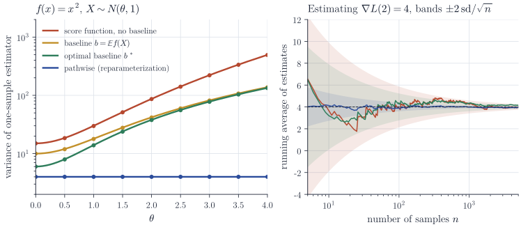
Variance of four gradient estimators as a function of theta on a log scale, and running averages of three estimators converging to the true gradient — Figure 1. Gradient of $\E X^2$ for $X \sim N(\theta, 1)$. Left: variance of the single-sample estimators; curves are the exact formulas, points are empirical variances from $2 \times 10^5$ draws. Right: running averages of the score-function estimator without baseline (red), with the optimal baseline (green), and of the pathwise estimator (blue) at $\theta = 2$, all computed from the same normal draws, with bands of two theoretical standard errors.

The pathwise estimator wins in this example by a wide margin, and this is typical when $f$ is smooth and the distribution is reparameterizable, though it is not a theorem: the pathwise variance depends on the size of $f'$, and examples exist where it is larger. The score-function estimator remains the general tool for discrete distributions, for non-differentiable or black-box $f$, and for problems such as policy gradients where $f$ depends on an environment that cannot be differentiated.

Remarks

The estimator in reinforcement learning is due to Williams (“Simple statistical gradient-following algorithms for connectionist reinforcement learning”, Machine Learning, 1992), and in discrete-event simulation to Glynn (“Likelihood ratio gradient estimation for stochastic systems”, Communications of the ACM, 1990), among others. Black-box variational inference (Ranganath, Gerrish and Blei, 2014) combines it with Rao–Blackwellization and control variates. The survey by Mohamed, Rosca, Figurnov and Mnih, “Monte Carlo gradient estimation in machine learning” (Journal of Machine Learning Research, 2020), compares the score-function, pathwise and measure-valued estimators in detail.