Score matching: fitting unnormalized densities without their normalizing constant
Many statistical models are specified through an unnormalized density
\[p_\theta(x) = \frac{q_\theta(x)}{Z(\theta)}, \qquad Z(\theta) = \int q_\theta(x)\, \dd x ,\]where \(q_\theta\) is easy to evaluate and \(Z(\theta)\) is an intractable integral: Markov random fields, energy-based models, exponential families with high-dimensional sufficient statistics, densities on manifolds. Maximum likelihood needs \(\log Z(\theta)\) or its gradient \(\nabla\log Z(\theta) = \E_\theta \nabla_\theta \log q_\theta(X)\), an expectation under the model that typically requires MCMC inside every optimization step.
Score matching, proposed by Hyvärinen (“Estimation of non-normalized statistical models by score matching”, Journal of Machine Learning Research, 2005), avoids \(Z\) entirely. It works with the gradient of the log density with respect to the data,
\[\psi_\theta(x) = \nabla_x \log p_\theta(x) = \nabla_x \log q_\theta(x),\]which does not depend on \(Z(\theta)\) because the normalizer is constant in \(x\). Here, as in that literature, “score” means this gradient in \(x\), not the gradient in \(\theta\) that appears in likelihood theory.
The Fisher divergence
Let the data have a density \(p\) on \(\R^d\) that is positive and continuously differentiable, with score \(\psi(x) = \nabla \log p(x)\). The natural criterion is the expected squared distance between model and data scores,
\[J(\theta) = \frac12 \E_p \bigl\lVert \psi_\theta(X) - \psi(X) \bigr\rVert^2 ,\]called the Fisher divergence. It vanishes when \(p_\theta = p\). Conversely, if \(J(\theta) = 0\) then \(\nabla \log p_\theta = \nabla\log p\) almost everywhere, hence everywhere by continuity; on the connected set \(\R^d\) the difference \(\log p_\theta - \log p\) is then constant, and since both densities integrate to one the constant is zero. So, for a correctly specified and identifiable model with positive densities, \(\theta_0\) is the unique minimizer of \(J\).
The objective contains the unknown data score \(\psi\), and estimating \(\psi\) nonparametrically would defeat the purpose. The cross term, however, can be rewritten without it.
Removing the data score
The argument is given for \(d = 1\). In \(d\) dimensions it is applied to each coordinate \(i\) in turn, with the other coordinates held fixed and Fubini’s theorem used to integrate over them; the integrability conditions are then imposed on \(\psi_{\theta,i}\), \(\psi_i\) and \(\partial_i\psi_{\theta,i}\), and the boundary condition becomes \(p(x)\psi_{\theta,i}(x) \to 0\) as \(x_i \to \pm\infty\) along almost every line parallel to the \(i\)th axis.
Theorem 1 (Hyvärinen). Let \(d = 1\), let \(p > 0\) and \(q_\theta > 0\) be continuously differentiable with \(\psi_\theta\) continuously differentiable, and assume
- \(\E_p \psi_\theta(X)^2 < \infty\), \(\E_p \psi(X)^2 < \infty\) and \(\E_p \abs{\psi_\theta'(X)} < \infty\);
- \(p(x)\psi_\theta(x) \to 0\) as \(x \to \pm\infty\).
Then
\[J(\theta) = \E_p\Bigl[\psi_\theta'(X) + \tfrac12 \psi_\theta(X)^2\Bigr] + \tfrac12 \E_p \psi(X)^2 .\]Proof. Expanding the square, which is legitimate because both scores are in \(L^2(p)\),
\[J(\theta) = \tfrac12 \E_p \psi_\theta^2 - \E_p[\psi_\theta \psi] + \tfrac12 \E_p\psi^2 .\]Since \(\psi = p'/p\), the middle expectation is \(\int \psi_\theta(x) p'(x)\, \dd x\); the integrand is integrable by the Cauchy–Schwarz inequality, because \(\E_p\abs{\psi_\theta\psi} \le (\E_p\psi_\theta^2\, \E_p\psi^2)^{1/2}\). For \(a < b\), integration by parts gives
\[\int_a^b \psi_\theta(x)\, p'(x)\, \dd x = \psi_\theta(b) p(b) - \psi_\theta(a) p(a) - \int_a^b \psi_\theta'(x)\, p(x)\, \dd x .\]Let \(a \to -\infty\) and \(b \to \infty\). The left side converges to \(\int \psi_\theta p'\) and the last integral to \(\E_p\psi_\theta'\), by dominated convergence and assumption 1; the boundary terms vanish by assumption 2. Hence \(\E_p[\psi_\theta \psi] = -\E_p \psi_\theta'\), and substituting gives the claim.
The last term does not depend on \(\theta\). Minimizing \(J\) is therefore equivalent to minimizing
\[\tilde J(\theta) = \E_p\Bigl[\sum_{i=1}^d \Bigl(\partial_i \psi_{\theta, i}(X) + \tfrac12 \psi_{\theta,i}(X)^2\Bigr)\Bigr],\]and its empirical version \(\tilde J_n(\theta)\), the average of the bracket over the observations \(X_1, \dots, X_n\), involves only \(q_\theta\) and its first two derivatives in \(x\). The score matching estimator \(\hat\theta_n\) minimizes \(\tilde J_n\). It is an M-estimator, so the usual arguments give consistency and asymptotic normality under regularity conditions; Hyvärinen (2005) gives a consistency argument for identifiable models.
The second derivative term is what replaces the data score. Intuitively, a good model should place the data at local maxima of \(\log q_\theta\), where the score is small and its derivative is negative, and the objective rewards exactly that. The boundary condition matters: for a density on a half-line or an interval, the boundary terms do not vanish in general, and the objective must be modified.
Exponential families: a linear system
Suppose \(\log q_\theta(x) = \theta^\top T(x) + b(x)\) with \(T : \R \to \R^k\) and \(b\) twice continuously differentiable. Then \(\psi_\theta = \theta^\top T' + b'\) and \(\psi_\theta' = \theta^\top T'' + b''\), so the empirical objective is a quadratic function of \(\theta\),
\[\tilde J_n(\theta) = \tfrac12 \theta^\top \hat A\, \theta + \theta^\top \hat c + \text{const},\]with
\[\hat A = \frac1n\sum_{i} T'(X_i) T'(X_i)^\top, \qquad \hat c = \frac1n \sum_i \bigl(T''(X_i) + b'(X_i) T'(X_i)\bigr).\]If \(\hat A\) is positive definite, \(\hat\theta_n = -\hat A^{-1} \hat c\): no integration, no optimization and no sampling. This is the setting in which score matching is most attractive, and its large-sample behaviour can be read off directly.
Proposition 2. In the exponential family above, suppose \(p = p_{\theta_0}\) satisfies the assumptions of Theorem 1 for every \(\theta\), that \(A = \E T'(X) T'(X)^\top\) is positive definite, and that \(\phi(x) = T'(x) T'(x)^\top \theta_0 + T''(x) + b'(x) T'(x)\) has \(\E\norm{\phi(X)}^2 < \infty\). Then
\[\sqrt n\,(\hat\theta_n - \theta_0) \xrightarrow{d} N\bigl(0,\; A^{-1} V A^{-1}\bigr), \qquad V = \Cov \phi(X).\]Proof. The population objective is \(\tilde J(\theta) = \tfrac12 \theta^\top A \theta + \theta^\top c + \text{const}\) with \(c = \E[T'' + b' T']\), and by Theorem 1 and the identification argument it is minimized at \(\theta_0\), so \(A\theta_0 + c = \E\phi(X) = 0\). Since \(\hat A\theta_0 + \hat c = n^{-1}\sum_i \phi(X_i)\),
\[\hat\theta_n - \theta_0 = -\hat A^{-1}\bigl(\hat A \theta_0 + \hat c\bigr) = -\hat A^{-1}\, \frac1n \sum_{i=1}^n \phi(X_i)\]whenever \(\hat A\) is invertible, which holds with probability tending to one because \(\hat A \to A\) almost surely. The central limit theorem applies to the average of the mean-zero vectors \(\phi(X_i)\), and Slutsky’s lemma gives the result.
The sandwich form \(A^{-1} V A^{-1}\) is that of an M-estimator whose objective is not a log-likelihood. Under the usual regularity conditions it is at least the inverse Fisher information, the asymptotic variance of maximum likelihood, in the positive semidefinite order, by the information inequality for unbiased estimating equations; equality holds in special cases such as the Gaussian family below.
For the Gaussian family, \(\log q_\theta(x) = -(x - m)^2/(2v)\) gives \(\psi_\theta(x) = -(x - m)/v\) and \(\psi_\theta' = -1/v\), so
\[\tilde J_n(m, v) = \frac{1}{2v^2}\cdot\frac1n\sum_i (X_i - m)^2 - \frac1v .\]The minimizer is \(\hat m = \bar X\) and \(\hat v = n^{-1}\sum_i (X_i - \bar X)^2\), the maximum likelihood estimator. This coincidence does not persist beyond simple cases.
A bimodal example
Consider the family
\[q_\theta(x) = \exp\Bigl(-\theta_1 \frac{x^2}{2} - \theta_2 \frac{x^4}{4}\Bigr), \qquad \theta_2 > 0 ,\]which is bimodal when \(\theta_1 < 0\). Its normalizer has no closed form. With \(T(x) = (-x^2/2, -x^4/4)\) and \(b = 0\), we have \(T'(x) = (-x, -x^3)\) and \(T''(x) = (-1, -3x^2)\), so, writing \(\hat m_k = n^{-1}\sum_i X_i^k\),
\[\hat\theta_n = \begin{pmatrix} \hat m_2 & \hat m_4 \\ \hat m_4 & \hat m_6 \end{pmatrix}^{-1} \begin{pmatrix} 1 \\ 3 \hat m_2 \end{pmatrix}.\]The matrix is a Gram matrix of the functions \(x\) and \(x^3\) under the empirical distribution and is positive definite as soon as the sample has at least two distinct nonzero absolute values. The assumptions of Theorem 1 hold for every \(\theta\) with \(\theta_2 > 0\), because \(p\) decays like \(e^{-x^4/4}\) and the scores are polynomials.
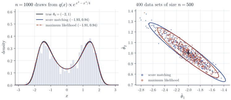
In one dimension the normalizer can be computed by quadrature, so maximum likelihood is available for comparison, and Figure 1 shows the two side by side. Both estimators recover the parameter, and the fitted densities are indistinguishable by eye. Over the \(400\) replications, the variances of the score matching estimates of \(\theta_1\) and \(\theta_2\) exceed those of maximum likelihood by factors of about \(1.6\) and \(1.4\). Proposition 2 predicts the same factors: computing \(A\), \(V\) and the Fisher information by quadrature gives ratios of asymptotic variances of \(1.57\) and \(1.41\). This loss of efficiency is the expected price: maximum likelihood is asymptotically efficient in a regular model, and score matching uses less information about the model, namely only its local shape. The strong negative correlation between \(\hat\theta_1\) and \(\hat\theta_2\) reflects the fact that the two terms trade off in determining the location of the modes.
Remarks
Several extensions keep the same idea. Hyvärinen (“Some extensions of score matching”, Computational Statistics and Data Analysis, 2007) adapts the objective to nonnegative data, where the boundary term at zero must be handled. Vincent (“A connection between score matching and denoising autoencoders”, Neural Computation, 2011) shows that matching the score of a noise-perturbed data distribution is equivalent to a denoising objective, which requires no second derivatives. Estimating the scores of the data distribution at many noise levels, by neural networks trained with this denoising objective, is the basis of score-based generative models and diffusion models, where the learned scores drive a sampler; Song and Ermon, “Generative modeling by estimating gradients of the data distribution” (NeurIPS, 2019), is an early example.