Margins and dependence, separated: copulas and Sklar’s theorem

A joint distribution mixes two kinds of information: how each coordinate behaves on its own, and how the coordinates move together. A correlation coefficient tries to summarize the second, but it is contaminated by the first. If $X$ and $Y$ are positively dependent and we replace $X$ by $e^X$, nothing about their joint ordering changes, yet the Pearson correlation does. A copula removes the marginal information completely. Transform each coordinate by its own distribution function so that it becomes uniform on $(0,1)$; the joint law of the transformed vector is the copula, and Sklar’s theorem says that the margins and the copula together recover the original distribution.

Throughout, a distribution function on $\R$ is nondecreasing, right-continuous, with limits $0$ and $1$ at $\mp\infty$, and inequalities between vectors are coordinatewise.

Quantile functions

For a distribution function $F$ define the quantile function

\[F^{-1}(u) = \inf\{x \in \R : F(x) \ge u\}, \qquad u \in (0,1).\]

The infimum is finite because $F$ has limits $0$ and $1$. The basic fact is the equivalence

\[\begin{equation} F^{-1}(u) \le x \iff u \le F(x), \qquad u \in (0,1),\ x \in \R . \label{eq:galois} \end{equation}\]

If $u \le F(x)$ then $x$ belongs to the set in the definition, so $F^{-1}(u) \le x$. Conversely, by right-continuity the set $\{x : F(x) \ge u\}$ is the closed half-line $[F^{-1}(u), \infty)$, so $F^{-1}(u) \le x$ implies $F(x) \ge u$.

Lemma 1. Let $U \sim \mathrm{Uniform}(0,1)$ and let $F$ be a distribution function.

$F^{-1}(U)$ has distribution function $F$.
If $F$ is continuous and $X \sim F$, then $F(X) \sim \mathrm{Uniform}(0,1)$ and $F^{-1}(F(X)) = X$ almost surely.

Proof. Part 1 follows from $\eqref{eq:galois}$: $\P(F^{-1}(U) \le x) = \P(U \le F(x)) = F(x)$.

For part 2, first note that $F(F^{-1}(u)) = u$ for $u \in (0,1)$: the inequality $\ge$ holds by right-continuity, and $F(x) < u$ for all $x < F^{-1}(u)$ gives $\le$ by continuity. By $\eqref{eq:galois}$, $\{F(X) \ge u\} = \{X \ge F^{-1}(u)\}$, and since $F$ is continuous,

\[\P(F(X) \ge u) = 1 - F\bigl(F^{-1}(u)\bigr) = 1 - u, \qquad u \in (0,1),\]

so $F(X)$ is uniform. Finally, $F^{-1}(F(X)) \le X$ always, and strict inequality means that $F$ is constant on an interval $[a, X]$ with $a < X$. The maximal intervals of constancy of $F$ with positive length are disjoint, hence countably many, and each carries probability zero under $F$; so strict inequality has probability zero.

Sklar’s theorem

A $d$-dimensional copula is the distribution function $C$ of a random vector $U = (U_1, \dots, U_d)$ whose coordinates are each $\mathrm{Uniform}(0,1)$. Every copula is Lipschitz: for $u, v \in [0,1]^d$, the events $\{U \le u\}$ and $\{U \le v\}$ differ only on the union of the events that $U_j$ lies between $u_j$ and $v_j$, so

\[\abs{C(u) - C(v)} \le \sum_{j=1}^d \abs{u_j - v_j} .\]

Theorem 2 (Sklar). Let $F_1, \dots, F_d$ be distribution functions on $\R$.

For every copula $C$, the function $H(x) = C\bigl(F_1(x_1), \dots, F_d(x_d)\bigr)$ is a joint distribution function with margins $F_1, \dots, F_d$.
If $H$ is a joint distribution function with continuous margins $F_1, \dots, F_d$, there is exactly one copula $C$ with $H(x) = C\bigl(F_1(x_1), \dots, F_d(x_d)\bigr)$ for all $x \in \R^d$, namely the distribution function of $(F_1(X_1), \dots, F_d(X_d))$ for $X \sim H$. It satisfies $C(u) = H\bigl(F_1^{-1}(u_1), \dots, F_d^{-1}(u_d)\bigr)$ for $u \in (0,1)^d$.

Proof. For part 1, let $U \sim C$ and $X_j = F_j^{-1}(U_j)$. By $\eqref{eq:galois}$ applied in each coordinate,

\[\P(X \le x) = \P\bigl(U_j \le F_j(x_j) \text{ for all } j\bigr) = C\bigl(F_1(x_1), \dots, F_d(x_d)\bigr),\]

and $X_j \sim F_j$ by Lemma 1.

For part 2, let $X \sim H$ and $U_j = F_j(X_j)$. By Lemma 1, each $U_j$ is uniform, so the distribution function $C$ of $U$ is a copula, and $X_j = F_j^{-1}(U_j)$ almost surely. The computation of part 1 then gives $H(x) = C(F_1(x_1), \dots, F_d(x_d))$. For uniqueness, suppose a copula $C'$ also represents $H$. Each $F_j$ is continuous, so its range contains $(0,1)$, and $C' = C$ on $(0,1)^d$; both are continuous, hence they agree on $[0,1]^d$. The last formula follows by substituting $x_j = F_j^{-1}(u_j)$ and using $F_j(F_j^{-1}(u_j)) = u_j$, shown in the proof of Lemma 1.

With discontinuous margins a copula representing $H$ still exists, but it is determined only on the product of the ranges of the $F_j$. For integer-valued data these ranges are countable sets, and many copulas give the same joint distribution. This makes copula modelling of count data delicate; C. Genest and J. Nešlehová, “A primer on copulas for count data” (ASTIN Bulletin, 2007), discuss the consequences.

The proof of part 1 is also a simulation algorithm: to sample from $H$, sample $U$ from the copula and apply the marginal quantile functions. The figure below was produced this way.

What a copula determines

Because $C$ is the law of the vector of ranks on the probability scale, it is unchanged by any increasing transformation of the coordinates.

Proposition 3. Suppose $X$ has continuous margins and copula $C$, and $g_1, \dots, g_d$ are strictly increasing functions on $\R$. Then $(g_1(X_1), \dots, g_d(X_d))$ also has copula $C$.

Proof. Let $Y_j = g_j(X_j)$ and let $X_j'$ be an independent copy of $X_j$. Since $g_j$ is injective, $\P(Y_j = y) \le \sup_x \P(X_j = x) = 0$, so $Y_j$ has a continuous distribution function $G_j$. Because $g_j$ is strictly increasing, $g_j(X_j') \le g_j(x) \iff X_j' \le x$, so $G_j(g_j(x)) = F_j(x)$ for every $x$. Hence $G_j(Y_j) = F_j(X_j)$, and the vectors that define the two copulas in Theorem 2 coincide.

Rank-based dependence measures are therefore functionals of the copula alone. Kendall’s tau, defined for an independent copy $(X', Y')$ of $(X, Y)$ as the probability of concordance minus the probability of discordance,

\[\tau = \P\bigl((X - X')(Y - Y') > 0\bigr) - \P\bigl((X - X')(Y - Y') < 0\bigr),\]

depends on $(X, Y)$ only through $C$, and for continuous margins it equals $4\,\E\,C(U, V) - 1$ with $(U, V) \sim C$. Pearson’s correlation is not a functional of the copula.

Copulas are also confined between two extremes.

Proposition 4 (Fréchet–Hoeffding bounds). Every $d$-dimensional copula satisfies

\[\max\Bigl(\sum_{j=1}^d u_j - d + 1,\ 0\Bigr) \le C(u) \le \min_j u_j\]

for all $u \in [0,1]^d$.

Proof. With $U \sim C$, $C(u) \le \P(U_j \le u_j) = u_j$ for each $j$. For the lower bound, by the union bound $1 - C(u) = \P\bigl(\bigcup_j \{U_j > u_j\}\bigr) \le \sum_j (1 - u_j)$.

The upper bound is the copula of $(U, U, \dots, U)$, perfect positive dependence. For $d = 2$ the lower bound is the copula of $(U, 1 - U)$, perfect negative dependence; for $d \ge 3$ it is not a copula, since it would assign the box $[1/2, 1]^d$ the probability $\sum_{k=0}^{d} (-1)^{k} \binom{d}{k} \max\bigl(1 - k/2, 0\bigr) = 1 - d/2 < 0$ (only the terms $k = 0, 1$ are nonzero; $k$ counts the coordinates set to $1/2$). The lower bound is nevertheless sharp pointwise: for each fixed $u$ some copula attains it.

Three copulas with the same Kendall’s tau

Two parametric families illustrate how much the copula leaves open once a summary such as $\tau$ is fixed.

The Gaussian copula with correlation $\rho$ is the copula of a bivariate normal vector, $C_\rho(u,v) = \Phi_{2,\rho}\bigl(\Phi^{-1}(u), \Phi^{-1}(v)\bigr)$, where $\Phi_{2,\rho}$ is the standard bivariate normal distribution function with correlation $\rho$. Its Kendall’s tau is $\tau = (2/\pi)\arcsin\rho$.

The Clayton copula with parameter $\theta > 0$ is

\[C_\theta(u, v) = \bigl(u^{-\theta} + v^{-\theta} - 1\bigr)^{-1/\theta},\]

with $\tau = \theta/(\theta + 2)$. It can be sampled by a construction of Marshall and Olkin: draw $V \sim \mathrm{Gamma}(1/\theta, 1)$ and independent $E_1, E_2 \sim \mathrm{Exp}(1)$, and set $U_j = (1 + E_j/V)^{-1/\theta}$. Indeed, conditionally on $V$, $\P(U_j \le u_j) = \P\bigl(E_j \ge V(u_j^{-\theta} - 1)\bigr) = \exp\{-V(u_j^{-\theta} - 1)\}$, the two events are conditionally independent, and averaging over $V$ with the Laplace transform $\E e^{-sV} = (1 + s)^{-1/\theta}$ gives

\[\P(U_1 \le u_1, U_2 \le u_2) = \bigl(1 + (u_1^{-\theta} - 1) + (u_2^{-\theta} - 1)\bigr)^{-1/\theta} = C_\theta(u_1, u_2).\]

The survival Clayton copula is the law of $(1 - U_1, 1 - U_2)$. The map $(u, v) \mapsto (1-u, 1-v)$ preserves concordance, so it has the same $\tau$.

The families differ in their tails. The lower tail dependence coefficient $\lambda_L = \lim_{u \downarrow 0} C(u,u)/u$ measures the probability that one coordinate is extremely small given that the other is. For Clayton, $C_\theta(u, u) = u\,(2 - u^\theta)^{-1/\theta}$, so $\lambda_L = 2^{-1/\theta}$; its survival version has the same coefficient in the upper tail. For the Gaussian copula with $\abs{\rho} < 1$ both tail coefficients are zero.

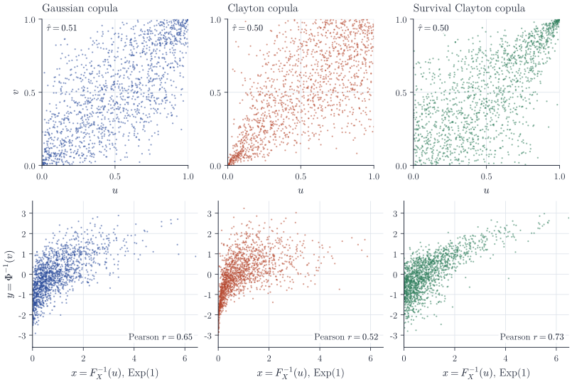
Scatter plots of three copulas with Kendall's tau 0.5 on the unit square, and the same samples after transforming to exponential and normal margins — Figure 1. Top: 1,500 draws from the Gaussian ($\rho = \sin(\pi/4)$), Clayton ($\theta = 2$) and survival Clayton ($\theta = 2$) copulas, all with $\tau = 0.5$. Clayton concentrates in the lower-left corner and its survival version in the upper-right corner. Bottom: the same draws after applying $F_X^{-1}$ for an $\mathrm{Exp}(1)$ margin and $\Phi^{-1}$ for a standard normal margin. The margins are identical across columns and so is $\tau$, while the Pearson correlations differ.

Figure 1 sets $\tau = 0.5$, that is, $\rho = \sin(\pi/4) \approx 0.71$ and $\theta = 2$, so that both Clayton copulas have tail coefficient $2^{-1/2} \approx 0.71$ in their dependent corner. In the bottom row, with the same exponential and normal margins in every column, the joint distributions differ visibly, and so do the sample Pearson correlations ($0.65$, $0.52$ and $0.73$). Knowing the margins and a rank correlation does not determine the joint distribution; the copula carries exactly the missing information.

Remarks

The decomposition is most useful when margins and dependence are estimated separately, for instance by fitting each margin (or using empirical distribution functions, which gives pseudo-observations $R_{ij}/(n+1)$, where $R_{ij}$ is the rank of the $i$th observation among the $n$ values of coordinate $j$) and then fitting a copula family to the transformed data. Sklar’s theorem guarantees that the combination is a valid joint distribution, and Proposition 3 explains why rank-based procedures are natural at the second stage.

R. B. Nelsen, An Introduction to Copulas, is the standard reference for the theory, including Sklar’s theorem for general margins. A. J. McNeil, R. Frey and P. Embrechts, Quantitative Risk Management, treat copulas with an emphasis on tail dependence and its consequences for risk aggregation.