Slice sampling: uniform draws under the graph of a density

October 12, 2026Computation

Many samplers need a tuning parameter whose wrong value makes them fail silently: a random-walk proposal that is too small, an importance density with light tails. Slice sampling, introduced in its general form by Neal (“Slice sampling”, Annals of Statistics, 2003), has a tuning parameter as well, but it affects only the cost of each update, and the update adapts to the local scale of the density on its own. The construction rests on a simple geometric fact, and its correctness on a symmetry argument given in full below.

The region under the graph

Let \(f : \R^d \to [0, \infty)\) be measurable with \(0 < Z = \int f(x)\, \dd x < \infty\). We can evaluate \(f\) but not \(Z\), and want draws from the density \(f/Z\). Define the region under the graph

\[G = \bigl\{(x, u) \in \R^d \times \R : 0 < u < f(x)\bigr\}.\]

Lemma 1. \(G\) has Lebesgue measure \(Z\). If \((X, U)\) is uniformly distributed on \(G\), then \(X\) has density \(f/Z\), and conditionally on \(X = x\) the variable \(U\) is uniform on \((0, f(x))\). Conversely, if \(X\) has density \(f/Z\) and \(U \mid X = x \sim \mathrm{U}(0, f(x))\), then \((X, U)\) is uniform on \(G\).

Proof. \(G\) is measurable because \((x, u) \mapsto f(x) - u\) is. By Tonelli’s theorem its measure is \(\int \int \mathbf 1\{0 < u < f(x)\}\, \dd u\, \dd x = \int f(x)\, \dd x = Z\). The uniform density on \(G\) is \(\mathbf 1_G(x, u)/Z\); integrating out \(u\) gives \(f(x)/Z\), and dividing the joint density by this marginal gives \(\mathbf 1\{0 < u < f(x)\}/f(x)\). The converse follows by multiplying the same two densities.

Lemma 1 is the basis of rejection sampling, which draws uniformly from a larger region containing \(G\) and keeps the points that land in \(G\). Slice sampling draws from \(G\) by a Markov chain instead. The two conditionals of the uniform distribution on \(G\) are

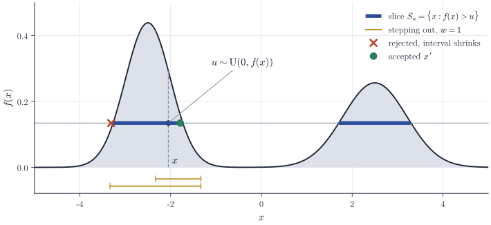
\[U \mid X = x \;\sim\; \mathrm{U}\bigl(0, f(x)\bigr), \qquad X \mid U = u \;\sim\; \mathrm{U}(S_u), \qquad S_u = \{x : f(x) > u\},\]

so alternating the two is a Gibbs sampler with invariant distribution uniform on \(G\), and its \(X\)-coordinate has invariant density \(f/Z\). The set \(S_u\) is the slice at level \(u\). It has finite measure for \(u > 0\), since \(\abs{S_u} \le Z/u\) by Markov’s inequality, and it contains the current point \(x\) because \(u < f(x)\).

The first conditional is trivial to sample. The second is not: the slice is defined implicitly, and for a multimodal \(f\) it may consist of several intervals whose endpoints are unknown. The rest of the note is about replacing the exact draw from \(\mathrm U(S_u)\) by a Markov update that leaves \(\mathrm U(S_u)\) invariant, which is all the Gibbs argument requires.

Stepping out and shrinkage

From now on \(d = 1\). Assume that \(f\) is continuous, so that every slice is open, and that \(f(x) \to 0\) as \(\abs{x} \to \infty\), so that every slice with \(u > 0\) is bounded. Fix a width \(w > 0\). Given the current point \(x\) and the level \(u\):

1. Stepping out. Draw \(V \sim \mathrm U(0, 1)\) and set \(L = x - wV\), \(R = L + w\). While \(f(L) > u\), replace \(L\) by \(L - w\). While \(f(R) > u\), replace \(R\) by \(R + w\).
2. Shrinkage. Draw \(y \sim \mathrm U(L, R)\). If \(f(y) > u\), return \(x' = y\). Otherwise set \(L = y\) if \(y < x\) and \(R = y\) if \(y > x\), and repeat.

Both loops terminate. Stepping out stops after finitely many steps because the slice is bounded and every endpoint at which the loop continues lies in it. For shrinkage, \(x\) stays in the interior of \((L, R)\), and since \(S_u\) is open there is \(\delta > 0\) with \((x - \delta, x + \delta) \subseteq S_u\). If \((L, R) \subseteq (x - \delta, x + \delta)\) the next draw is accepted; otherwise \((L, R) \cap (x-\delta, x+\delta)\) has length at least \(\delta\), so the next draw is accepted with probability at least \(\delta/(R_0 - L_0)\), where \((L_0, R_0)\) is the interval produced by stepping out. The number of shrinkage steps is therefore dominated by a geometric random variable. In code:

def slice_step(x, f, w, rng):
    u = rng.uniform(0, f(x))
    L = x - w * rng.random(); R = L + w
    while f(L) > u: L -= w
    while f(R) > u: R += w
    while True:
        y = rng.uniform(L, R)
        if f(y) > u:
            return y
        if y < x: L = y
        else:     R = y

Figure 1. One update for $f(x) = 0.55\,\phi_{0.5}(x + 2.5) + 0.45\,\phi_{0.7}(x - 2.5)$, with $\phi_s$ the $N(0, s^2)$ density. The level $u$ cuts the density in two intervals (blue). Stepping out with $w = 1$ (gold, one row per stage) stops at grid points outside the slice and never reaches the right component. One proposal falls outside the slice and shrinks the interval; the next is accepted (green).

Why the procedure is exact

Write \(S = S_u\) for a fixed level and let \(k(x, \cdot)\) be the distribution of \(x'\) produced by the two loops from \(x \in S\). It has a density, also denoted \(k(x, x')\), supported on \(S\).

Theorem 2. Under the assumptions above, \(k(x, x') = k(x', x)\) for almost every \(x, x' \in S\). Consequently \(k\) is reversible with respect to the uniform distribution on \(S\), and the slice sampler, which draws \(u \sim \mathrm U(0, f(x))\) and then \(x' \sim k(x, \cdot)\) for the slice at level \(u\), leaves \(f/Z\) invariant.

Proof. Stepping out depends on \(x\) only through a random grid. The endpoints visited are points of \(\Gamma = L + w\Z\), where \(L = x - wV\). The position of this grid modulo \(w\) is uniform on \([0, w)\) whatever \(x\) is, so \(\Gamma\) has the same law for every starting point. Given \(\Gamma\), the loop returns the interval \(I(x, \Gamma) = (a, b)\), where \(a\) is the largest point of \(\Gamma\) to the left of \(x\) that is not in \(S\) and \(b\) the smallest such point to its right; all grid points strictly between \(a\) and \(b\) lie in \(S\). If \(x' \in S \cap (a, b)\) is not a grid point, the same description applied to \(x'\) gives the same \(a\) and \(b\). Hence, for each grid, \(x' \in I(x, \Gamma)\) if and only if \(x \in I(x', \Gamma)\), and in that case \(I(x, \Gamma) = I(x', \Gamma)\).

Shrinkage is symmetric. Fix an interval \(I_0\) containing \(x\) and \(x'\). The density of returning \(x'\) after exactly \(m\) rejections at points \(y_1, \dots, y_m\) is

\[\prod_{j=1}^{m} \frac{\mathbf 1\{y_j \in I_{j-1} \setminus S\}}{\abs{I_{j-1}}} \cdot \frac{\mathbf 1\{x' \in I_m\}}{\abs{I_m}},\]

where \(I_j\) is obtained from \(I_{j-1}\) by cutting at \(y_j\) and keeping the side containing \(x\). If no \(y_j\) lies between \(x\) and \(x'\), each cut keeps the same side for \(x\) and for \(x'\), so the intervals, and hence the expression above, are the same with \(x\) and \(x'\) exchanged. If some \(y_j\) lies between them, the first such cut removes \(x'\) when shrinking toward \(x\) and removes \(x\) when shrinking toward \(x'\), so the expression vanishes in both directions. Integrating over \(y_1, \dots, y_m\) and summing over \(m\) gives \(p(x' \mid x, I_0) = p(x \mid x', I_0)\).

Combining the two steps, \(k(x, x') = \E_\Gamma\bigl[\mathbf 1\{x' \in I(x, \Gamma)\}\, p\bigl(x' \mid x, I(x, \Gamma)\bigr)\bigr]\), and the expectation is unchanged when \(x\) and \(x'\) are exchanged. A symmetric transition density is reversible with respect to the uniform distribution on \(S\). The final statement then follows as for any Gibbs sampler: the update of \(u\) is an exact conditional draw, and the update of \(x\) leaves the conditional distribution \(\mathrm U(S_u)\) of \(X\) given \(U = u\) invariant, so both leave the uniform distribution on \(G\) invariant, and Lemma 1 identifies its \(x\)-marginal.

Two features of the procedure are essential to this proof. The random offset \(V\) makes the grid independent of the starting point; with \(L = x - w/2\) fixed, the interval would depend on \(x\) in a way that breaks symmetry. And shrinkage must keep the side containing the current point, which is what makes a rejected point between \(x\) and \(x'\) exclude the move in both directions. Neal (2003) also treats a bounded number \(m\) of stepping-out steps, which remains exact if the budget is split at random between the two sides, and a doubling procedure, which needs an additional acceptance test.

The role of the width

Every \(w > 0\) gives a valid sampler, so \(w\) governs only efficiency. If \(w\) is much smaller than the slice, stepping out needs many evaluations of \(f\). If \(w\) is much larger, the first proposals are often rejected, but each rejection cuts the interval at the rejected point. When the slice occupies a small part of the interval, a rejected point is nearly uniform on the interval, and a cut at a uniform point keeps on average a fraction \(\tfrac12 + t - t^2 \le \tfrac34\) of it, where \(t\) is the relative position of \(x\); so the number of shrinkage steps grows roughly like \(\log w\). In this sense the method adapts its step to the local scale of \(f\), and in practice it is far less sensitive to its tuning parameter than random-walk Metropolis.

The exception is a slice with several components. Stepping out stops at the first grid point outside the slice, so when the gap between two modes is wider than \(w\) at the current level, the update cannot leave the current component. The chain can move between modes only at iterations where \(u\) is so low that the gap between the two components of the slice is narrower than \(w\) (or closed), which, starting from the bulk of a mode, has small probability. Figure 2 shows the consequence on the mixture of Figure 1.

Figure 2. Twenty thousand slice-sampling updates for the mixture of Figure 1, started at $x_0 = -2.5$, with $w = 0.3$ (top) and $w = 4$ (bottom). With the narrow width the chain crosses between the modes only about twenty times, so the estimated mass of the right component is far from $0.45$; with the wide width it switches constantly. The histograms compare the draws with the normalized target.

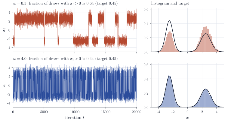
Both chains in Figure 2 have the correct invariant distribution and the narrow one will eventually produce the right proportions; it simply needs far more iterations.

Remarks

In several dimensions the univariate update can be applied to one coordinate at a time, or along a random direction through the current point, and each such update preserves the target by the argument above applied to the conditional density along the line. Elliptical slice sampling (Murray, Adams and MacKay, 2010) adapts the shrinkage idea to models with a Gaussian prior, shrinking an angle on an ellipse instead of an interval. Neal’s paper remains the reference for the full set of procedures and their proofs, including the multivariate hyperrectangle version and overrelaxed variants.