Stochastic variational inference: natural-gradient steps from minibatches
Coordinate ascent variational inference (CAVI) for a model with global and local latent variables alternates between updating every local factor and then the global factor. Each global update requires a pass over the whole data set, which is wasteful when the data are large and redundant: early in the optimization, the global parameters are poor, and refining every local factor against them is wasted work. Hoffman, Blei, Wang and Paisley (Stochastic variational inference, JMLR, 2013) observed that in conditionally conjugate models the CAVI update for the global parameter is a natural-gradient step of unit length, and that the natural gradient admits cheap unbiased estimates from subsamples. The derivation is short, and a Gaussian mixture shows what the resulting algorithm buys.
Model class
There are \(N\) observations \(x_{1:N}\), local latent variables \(z_{1:N}\), one for each observation, and a global latent variable \(\beta\). The joint density factorizes as
\[p(\beta, z_{1:N}, x_{1:N}) = p(\beta) \prod_{i=1}^N p(x_i, z_i \mid \beta).\]The model is conditionally conjugate in \(\beta\) if, for some sufficient statistic \(t(\beta)\) and base measure \(h\),
\[p(\beta) \propto h(\beta) \exp\{\alpha^\top t(\beta)\}, \qquad p(x_i, z_i \mid \beta) = g(x_i, z_i) \exp\bigl\{ f(x_i, z_i)^\top t(\beta) - c(\beta) \bigr\},\]where the last coordinate of \(t\) may be taken to be \(-c(\beta)\) so that the factor \(e^{-c(\beta)}\) is absorbed. The complete conditional of \(\beta\) is then in the exponential family generated by \(t\) and \(h\), with natural parameter
\[\eta(x, z) = \alpha + \sum_{i=1}^N f(x_i, z_i).\]The variational family is mean-field, \(q(\beta)\prod_i q(z_i)\), where \(q(\beta) = q(\beta\mid\lambda) = h(\beta)\exp\{\lambda^\top t(\beta) - a(\lambda)\}\) belongs to the same family, assumed regular and minimal, so that \(a\) is smooth and strictly convex on the open convex set \(\Lambda\) of natural parameters, with \(\nabla a(\lambda) = \E_\lambda t(\beta)\) and \(\nabla^2 a(\lambda) = \Cov_\lambda t(\beta)\) positive definite. The local factors \(q(z_i\mid\varphi_i)\) are arbitrary, and \(\bar f_i(\varphi_i) = \E_{\varphi_i} f(x_i, z_i)\) is assumed finite.
The natural gradient is the coordinate-ascent step
Write \(\mathcal L(\lambda, \varphi)\) for the ELBO. Since \(\log p(\beta, z, x) = \log p(\beta\mid x, z) + \log p(x, z)\) and the second term does not involve \(\beta\), the part of \(\mathcal L\) that depends on \(\lambda\) is
\[\E_q \log p(\beta \mid x, z) - \E_q \log q(\beta\mid\lambda) = \nabla a(\lambda)^\top \bigl(\bar\eta(\varphi) - \lambda\bigr) + a(\lambda) + \text{const},\]with \(\bar\eta(\varphi) = \alpha + \sum_{i=1}^N \bar f_i(\varphi_i)\). Here the \(h(\beta)\) terms cancel, the normalizer of \(p(\beta\mid x,z)\) is absorbed into the constant, and we used \(\E_q t(\beta) = \nabla a(\lambda)\) together with the independence of \(\beta\) and \(z\) under \(q\).
Proposition 1. For fixed \(\varphi\), the map \(\lambda \mapsto \mathcal L(\lambda, \varphi)\) has gradient \(\nabla_\lambda \mathcal L = \nabla^2 a(\lambda)\bigl(\bar\eta(\varphi) - \lambda\bigr)\) and is uniquely maximized at \(\lambda = \bar\eta(\varphi)\) whenever \(\bar\eta(\varphi) \in \Lambda\). The Fisher information of \(q(\cdot\mid\lambda)\) is \(\nabla^2 a(\lambda)\), so the natural gradient is
\[\widetilde\nabla_\lambda \mathcal L = \bigl(\nabla^2 a(\lambda)\bigr)^{-1} \nabla_\lambda \mathcal L = \bar\eta(\varphi) - \lambda .\]Proof. Differentiating the display, \(\nabla_\lambda\bigl[\nabla a(\lambda)^\top(\bar\eta - \lambda) + a(\lambda)\bigr] = \nabla^2 a(\lambda)(\bar\eta - \lambda) - \nabla a(\lambda) + \nabla a(\lambda)\). The gradient vanishes only at \(\lambda = \bar\eta\) because \(\nabla^2 a\) is positive definite. That this stationary point is the maximum follows from writing the \(\lambda\)-dependent part as \(-\mathrm{KL}\bigl(q(\cdot\mid\lambda)\Vert q(\cdot\mid\bar\eta)\bigr)\) plus a constant, which is a direct check using \(\mathrm{KL}(q_\lambda\Vert q_{\bar\eta}) = a(\bar\eta) - a(\lambda) - \nabla a(\lambda)^\top(\bar\eta - \lambda)\). For an exponential family in natural parameters the score is \(t(\beta) - \nabla a(\lambda)\), whose covariance is \(\nabla^2 a(\lambda)\).
A natural-gradient step with step size \(\rho\) is therefore \(\lambda \leftarrow (1-\rho)\lambda + \rho\,\bar\eta(\varphi)\). With \(\rho = 1\) it is the CAVI update; with \(\rho \in (0,1)\) and \(\bar\eta(\varphi) \in \Lambda\) it is a convex combination of two points of the convex set \(\Lambda\), so the iterate remains a valid natural parameter without any projection. The Euclidean gradient carries the extra factor \(\nabla^2 a(\lambda)\), which can be badly conditioned and changes under reparametrization of \(q\); the natural gradient is the steepest-ascent direction when distances between variational distributions are measured locally by the Kullback–Leibler divergence.
Subsampling
The local factors affect the gradient in \(\lambda\) only through \(\bar\eta\). Let \(\varphi_i^\ast(\lambda)\) denote the optimal local factor for observation \(i\) given the global parameter, and consider the profiled objective \(\bar{\mathcal L}(\lambda) = \mathcal L(\lambda, \varphi^\ast(\lambda))\). If \(\varphi^\ast\) is differentiable and each \(\varphi_i^\ast(\lambda)\) is an interior maximizer, so that \(\nabla_\varphi \mathcal L\) vanishes there, the chain rule gives \(\nabla \bar{\mathcal L}(\lambda) = \nabla_\lambda \mathcal L(\lambda, \varphi^\ast(\lambda))\), and by Proposition 1 the natural gradient of the profiled objective is
\[\widetilde\nabla \bar{\mathcal L}(\lambda) = \alpha + \sum_{i=1}^N \bar f_i\bigl(\varphi_i^\ast(\lambda)\bigr) - \lambda .\]This is a sum over observations, so it can be estimated by sampling. Draw a minibatch \(S \subseteq \{1,\dots,N\}\) of \(B\) indices uniformly with replacement, compute the local optima for those indices only, and set
\[\hat\eta = \alpha + \frac{N}{B} \sum_{i \in S} \bar f_i\bigl(\varphi_i^\ast(\lambda)\bigr).\]Then \(\E[\hat\eta \mid \lambda] = \bar\eta(\varphi^\ast(\lambda))\), so \(\hat\eta - \lambda\) is an unbiased estimate of the natural gradient. The convex-combination update below stays in \(\Lambda\) as long as each \(\hat\eta\) lies in \(\Lambda\), which holds in the example below. The estimate has a concrete interpretation: \(\hat\eta\) is the CAVI update that would be computed if the data set consisted of the minibatch replicated \(N/B\) times. Stochastic variational inference iterates
\[\lambda_{t+1} = (1 - \rho_t)\, \lambda_t + \rho_t\, \hat\eta_t, \qquad \sum_t \rho_t = \infty, \quad \sum_t \rho_t^2 < \infty,\]the step-size conditions being those of Robbins and Monro (A stochastic approximation method, Annals of Mathematical Statistics, 1951). A common choice is \(\rho_t = (t + \tau)^{-\kappa}\) with \(\kappa \in (1/2, 1]\) and a delay \(\tau \ge 0\) that damps the first steps. The first condition lets the iterates travel arbitrarily far. Unbiasedness makes the partial sums of the accumulated noise \(\sum_t \rho_t(\hat\eta_t - \E[\hat\eta_t\mid\lambda_t])\) a martingale, and the second condition, together with bounded conditional variances, makes this martingale bounded in \(L^2\) and hence almost surely convergent. Turning this into a convergence theorem for \(\lambda_t\) requires further conditions, such as bounded iterates and smoothness of \(\bar{\mathcal L}\), under which stochastic approximation theory yields convergence to a stationary point; Hoffman et al. discuss this.
Each step costs \(O(B)\) local updates, independent of \(N\). The price is noise: since \(\hat\eta\) scales the minibatch sum by \(N/B\), its variance is of order \(N^2/B\) times the variance of a single \(\bar f_i\), and only the decreasing step sizes average it out.
Example: a mixture with unknown means
Let \(\mu_1, \dots, \mu_K \in \R^d\) be independent with prior \(\mathcal N(0, \sigma_0^2 I_d)\), let \(z_i\) be uniform on \(\{1, \dots, K\}\), and let \(x_i \mid z_i, \mu \sim \mathcal N(\mu_{z_i}, I_d)\). Here \(\beta = (\mu_1, \dots, \mu_K)\), and with the statistic \(t(\mu_k) = (\mu_k, \norm{\mu_k}^2)\) for each component the model is conditionally conjugate:
\[\alpha_k = \Bigl(0, -\frac{1}{2\sigma_0^2}\Bigr), \qquad f_k(x_i, z_i) = \mathbb 1\{z_i = k\} \Bigl(x_i, -\frac12\Bigr).\]Take \(q(\mu_k) = \mathcal N(m_k, s_k^2 I_d)\), with natural parameter \(\lambda_k = \bigl(m_k/s_k^2, -1/(2s_k^2)\bigr)\), and categorical \(q(z_i) = (\varphi_{i1}, \dots, \varphi_{iK})\). The optimal local factor is
\[\varphi_{ik}^\ast \propto \exp\Bigl\{ x_i^\top m_k - \tfrac12\bigl(\norm{m_k}^2 + d\, s_k^2\bigr) \Bigr\},\]and the minibatch target is \(\hat\eta_k = \bigl( \tfrac{N}{B}\sum_{i\in S} \varphi_{ik}^\ast x_i,\; -\tfrac{1}{2\sigma_0^2} - \tfrac{N}{2B}\sum_{i\in S}\varphi_{ik}^\ast \bigr)\). Both coordinates of the update are averages of the old and new natural parameters; in particular the second coordinate stays negative, so \(s_k^2\) stays positive. The ELBO maximized over the local factors has the closed form
\[\bar{\mathcal L}(\lambda) = \sum_{i=1}^N \log \sum_{k=1}^K \frac1K \exp\bigl\{\E_q \log \phi_d(x_i - \mu_k)\bigr\} + \sum_{k=1}^K \Bigl( \E_q \log p(\mu_k) + H\bigl(q(\mu_k)\bigr) \Bigr),\]with \(\phi_d\) the standard normal density on \(\R^d\), and this is what Figure 1 tracks.
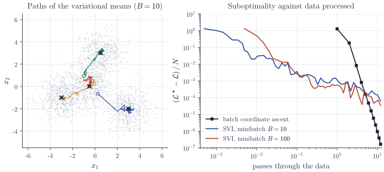
The right panel shows the trade-off. After a few percent of one pass, long before batch coordinate ascent has completed its first update, SVI with \(B = 10\) is within a few hundredths of a nat per observation of the optimum; the global parameters are determined by a small fraction of a redundant data set, and SVI exploits that. After that the stochastic iterates settle at a noise floor that decreases only as fast as the step sizes do, and batch coordinate ascent, whose error here decreases geometrically once it reaches the basin of the optimum, overtakes it after a few passes. Larger minibatches lower the noise per step at a proportional cost per step. In practice one combines the two regimes: run SVI while far from the optimum and then increase the minibatch size, average the iterates, or finish with batch updates.
Remarks
Conditional conjugacy is what makes the natural gradient free to compute; in non-conjugate models the same stochastic scheme applies with Monte Carlo gradient estimates of the ELBO, at the cost of an additional layer of noise. The local step can also be inexact, provided it increases \(\mathcal L\) for the sampled observations, but then the unbiasedness argument above no longer applies exactly. The subsampling identity requires the observations to enter the joint density as a product of factors with a common global parameter; for dependent data such as time series one must subsample blocks and account for the dependence between them. Amari, Natural gradient works efficiently in learning (Neural Computation, 1998), is the standard reference for natural gradients.