Variance as a power of the mean: Tweedie distributions

October 12, 2026Statistical theory

The four response distributions most used with generalized linear models have variance functions \(V(\mu) = 1, \mu, \mu^2, \mu^3\): normal, Poisson, gamma and inverse Gaussian. They are the cases \(p = 0, 1, 2, 3\) of the power law \(\Var Y = \phi \mu^p\). Tweedie (1984) and Jørgensen (1987) studied the whole class of exponential dispersion models with power variance functions, now called Tweedie distributions. The most useful new members are those with \(1 < p < 2\). They are continuous on \((0, \infty)\) but put positive probability on \(y = 0\), which is the shape of insurance claim totals, daily rainfall and biomass in ecological surveys. Below, the class is derived from its variance function, and the case \(1 < p < 2\) is identified as a compound Poisson distribution.

Exponential dispersion models

An exponential dispersion model is a family of distributions on \(\R\) with densities, with respect to a fixed measure, of the form

\[f(y; \theta, \phi) = a(y, \phi) \exp\Bigl\{ \frac{y\theta - \kappa(\theta)}{\phi} \Bigr\}, \qquad \theta \in \Theta, \; \phi > 0,\]

where \(\Theta\) is an open interval and the normalization \(\int a(y, \phi) e^{y\theta/\phi} \, \dd y = e^{\kappa(\theta)/\phi}\) holds for every \(\theta \in \Theta\) (for discrete families the integral is a sum). The function \(\kappa\) is the cumulant function.

Lemma 1. If \(Y\) has density \(f(\cdot\,; \theta, \phi)\), then for every \(t\) with \(\theta + \phi t \in \Theta\),

\[\log \E e^{tY} = \frac{\kappa(\theta + \phi t) - \kappa(\theta)}{\phi} .\]

Consequently \(\E Y = \kappa'(\theta)\) and \(\Var Y = \phi\, \kappa''(\theta)\).

Proof. \(\E e^{tY} = e^{-\kappa(\theta)/\phi} \int a(y, \phi) e^{y(\theta + \phi t)/\phi} \, \dd y = e^{(\kappa(\theta + \phi t) - \kappa(\theta))/\phi}\) by the normalization at \(\theta + \phi t\). Since \(\theta\) is interior to \(\Theta\), the cumulant generating function is finite near \(t = 0\), hence analytic there, and its first two derivatives at zero are the mean and the variance.

Because the variance is positive for a nondegenerate family, \(\kappa'' > 0\) and \(\mu = \kappa'(\theta)\) is a strictly increasing function of \(\theta\). Writing \(\theta\) as a function of \(\mu\) gives the variance function \(V(\mu) = \kappa''(\theta(\mu))\) and the mean–variance relation \(\Var Y = \phi V(\mu)\). Conversely, a variance function together with its domain of means determines the family (Morris, 1982, for natural exponential families; Jørgensen, 1997, for dispersion models). This is why it makes sense to define a family by prescribing \(V\).

Power variance functions

Suppose \(V(\mu) = \mu^p\) on \(\mu > 0\). From \(d\mu/d\theta = \kappa''(\theta) = V(\mu)\) and \(d\kappa/d\theta = \mu\),

\[\frac{d\theta}{d\mu} = \mu^{-p}, \qquad \frac{d\kappa}{d\mu} = \frac{d\kappa}{d\theta}\frac{d\theta}{d\mu} = \mu^{1-p} .\]

Integrating, and choosing the constants of integration to be zero (a constant added to \(\theta\) or to \(\kappa\) can be absorbed into \(a(y, \phi)\)),

\[\theta = \frac{\mu^{1-p}}{1 - p}, \qquad \kappa(\theta) = \frac{\mu^{2-p}}{2 - p} = \frac{\bigl((1 - p)\theta\bigr)^{(2-p)/(1-p)}}{2 - p}, \qquad p \ne 1, 2,\]

with \(\theta = \log\mu\), \(\kappa = e^\theta\) for \(p = 1\), and \(\theta = -1/\mu\), \(\kappa = -\log(-\theta)\) for \(p = 2\). The integration produces a candidate cumulant function; whether \(e^{\kappa(\theta)/\phi}\) is actually the Laplace transform of a measure has to be checked. The answer, due to Jørgensen, is:

• \(p = 0\): normal; \(p = 1\): Poisson (for \(\phi \ne 1\), \(Y/\phi\) is Poisson, so \(Y\) lives on the lattice \(\phi\N\)); \(p = 2\): gamma; \(p = 3\): inverse Gaussian;
• \(1 < p < 2\): compound Poisson sums of gamma variables, treated below;
• \(p > 2\), \(p \neq 3\): continuous distributions on \((0, \infty)\) generated by positive stable laws;
• \(p < 0\): continuous distributions on the whole real line, defined only for positive means;
• \(0 < p < 1\): no exponential dispersion model exists.

The negative result for \(0 < p < 1\) is not obvious from the variance function, which is perfectly regular there; see Jørgensen (1997) for the proof.

The compound Poisson case

Theorem 2. Let \(1 < p < 2\), \(\mu > 0\), \(\phi > 0\), and set

\[\lambda = \frac{\mu^{2-p}}{\phi(2 - p)}, \qquad \alpha = \frac{2 - p}{p - 1}, \qquad \gamma = \phi(p - 1)\mu^{p-1} .\]

Let \(N \sim \mathrm{Poisson}(\lambda)\) and, independently, let \(G_1, G_2, \dots\) be i.i.d. gamma variables with shape \(\alpha\) and scale \(\gamma\). Then \(Y = \sum_{j=1}^N G_j\) (with \(Y = 0\) when \(N = 0\)) has the Tweedie distribution with power \(p\), mean \(\mu\) and dispersion \(\phi\).

Proof. Conditioning on \(N\) and using \(\E e^{tG_1} = (1 - \gamma t)^{-\alpha}\) for \(t < 1/\gamma\),

\[\log \E e^{tY} = \log \E\bigl[(1 - \gamma t)^{-\alpha N}\bigr] = \lambda\bigl[(1 - \gamma t)^{-\alpha} - 1\bigr].\]

On the other side, \(1 < p < 2\) gives \(\theta = \mu^{1-p}/(1 - p) < 0\) and \(\Theta = (-\infty, 0)\). Since \(\kappa(\theta) = c\, \abs{\theta}^{-\alpha}\) for a constant \(c\) (the exponent \((2 - p)/(1 - p)\) equals \(-\alpha\)), Lemma 1 gives, for \(\theta + \phi t < 0\),

\[\frac{\kappa(\theta + \phi t) - \kappa(\theta)}{\phi} = \frac{\kappa(\theta)}{\phi}\Bigl[\Bigl(1 + \frac{\phi t}{\theta}\Bigr)^{-\alpha} - 1\Bigr] .\]

Now \(\kappa(\theta)/\phi = \mu^{2-p}/(\phi(2-p)) = \lambda\) and \(-\phi/\theta = \phi(p - 1)\mu^{p-1} = \gamma\), so the two cumulant generating functions agree on the interval \(t < 1/\gamma\), which contains a neighbourhood of zero. A cumulant generating function finite near zero determines the distribution. The calculation also settles existence in this range. Fix \(\phi\) and let \(\nu\) be the compound Poisson–gamma law built from some \(\theta_0 \in \Theta\). Tilting it, \(\nu_\theta(\dd y) = \exp\{[y(\theta - \theta_0) - \kappa(\theta) + \kappa(\theta_0)]/\phi\}\, \nu(\dd y)\), gives by the display above a probability measure with cumulant generating function \(\{\kappa(\theta + \phi t) - \kappa(\theta)\}/\phi\) for every \(\theta < 0\); so the laws \(\nu_\theta\), \(\theta \in \Theta\), form an exponential dispersion model with cumulant function \(\kappa\), and \(\nu_\theta\) is the compound Poisson–gamma law with the parameters of the theorem.

Several properties follow at once. The probability of an exact zero is

\[\P(Y = 0) = e^{-\lambda} = \exp\Bigl\{ -\frac{\mu^{2-p}}{\phi(2-p)} \Bigr\},\]

and on \((0, \infty)\) the distribution has the density

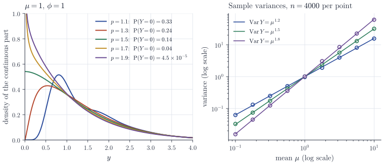
\[f(y) = \sum_{n=1}^\infty e^{-\lambda} \frac{\lambda^n}{n!} \cdot \frac{y^{n\alpha - 1} e^{-y/\gamma}}{\Gamma(n\alpha)\, \gamma^{n\alpha}} ,\]

a Poisson mixture of gamma densities. There is no closed form, but the series converges quickly for moderate \(\lambda\), and Dunn and Smyth (2005) give methods that work across the parameter space. The shape parameter \(\alpha\) of the summands depends only on \(p\). As \(p \downarrow 1\), \(\alpha \to \infty\) while the mean \(\alpha\gamma = \phi(2 - p)\mu^{p-1}\) of a summand tends to \(\phi\), so the summands concentrate at \(\phi\) and the law approaches the Poisson law on \(\phi\N\). As \(p \uparrow 2\), \(\lambda \to \infty\) and \(\alpha \to 0\): many tiny gamma pieces add up to a gamma variable, and the atom at zero disappears.

Figure 1. Left: the density of the continuous part of $Y$ for $\mu = 1$, $\phi = 1$, from the series above, with the atom $\mathrm{P}(Y = 0)$ in the legend. For $p = 1.1$ the summands are concentrated around their mean $0.9$, and the density has bumps near $y = 0.8$ and $y = 1.7$, the modes of one and of two summands. Right: sample variances of $4000$ simulated compound Poisson–gamma variables at nine means, on log-log axes; the lines have slope $p$.

Scale invariance

Proposition 3. If \(Y\) is Tweedie with power \(p\), mean \(\mu\) and dispersion \(\phi\), and \(c > 0\), then \(cY\) is Tweedie with power \(p\), mean \(c\mu\) and dispersion \(c^{2-p}\phi\).

Proof. Take \(p \ne 1, 2\); the two remaining cases are checked in the same way with their explicit \(\kappa\). The cumulant function satisfies \(\kappa(s\theta) = s^{(2-p)/(1-p)} \kappa(\theta)\) for \(s > 0\). Put \(\theta' = c^{1-p}\theta\), which is the canonical parameter of mean \(c\mu\), and \(\phi' = c^{2-p}\phi\). Then \(\theta' + \phi' t = c^{1-p}(\theta + c\phi t)\) and, by homogeneity,

\[\frac{\kappa(\theta' + \phi' t) - \kappa(\theta')}{\phi'} = \frac{c^{2-p}\bigl(\kappa(\theta + c\phi t) - \kappa(\theta)\bigr)}{c^{2-p}\phi} = \log \E e^{ctY},\]

which is the cumulant generating function of \(cY\).

Scale invariance is a practical requirement: a model for claim amounts should not depend on whether they are recorded in dollars or in thousands of dollars, and here a change of units only rescales the dispersion. Jørgensen showed that the Tweedie models are the only exponential dispersion models with this property, which is the deeper reason why power variance functions keep appearing in applications. In ecology the empirical regularity that log variance is linear in log mean across populations is known as Taylor’s power law (Taylor, 1961), and the right panel of Figure 1 is its simplest instance.

Tweedie regression

A Tweedie generalized linear model usually takes the log link, \(\log\mu_i = x_i^\top\beta\), with common power \(p\) and dispersion \(\phi\). For fixed \(p\) the score equations for \(\beta\) are

\[\sum_{i=1}^n \frac{y_i - \mu_i}{\mu_i^{p}} \, \mu_i x_i = \sum_{i=1}^n (y_i - \mu_i)\, \mu_i^{1-p} x_i = 0,\]

which do not involve \(\phi\) and do not require evaluating the density. The density is needed to estimate \(p\) and \(\phi\) by maximum likelihood, typically by profiling over a grid of \(p\) values.

Theorem 2 also explains a modelling restriction. The expected number of summands \(\lambda_i = \mu_i^{2-p}/(\phi(2-p))\) and the mean summand \(\alpha\gamma_i = \phi(2-p)\mu_i^{p-1}\) are both increasing in \(\mu_i\) when \(1 < p < 2\). In insurance language, a Tweedie regression with constant dispersion forces every covariate that raises expected cost to raise both claim frequency and claim severity. When the data suggest otherwise, letting \(\phi\) depend on covariates as well, in a double generalized linear model, removes the restriction.

Remarks

For \(p > 2\) the Tweedie densities are again series expansions, now derived from positive stable laws, and they are useful for very skewed positive data. For all \(p \ge 1\) the family contains distributions with support in \([0, \infty)\), and for all \(p\) the quasi-likelihood based on \(V(\mu) = \mu^p\) is available even when no Tweedie density is.

References: M. C. K. Tweedie, “An index which distinguishes between some important exponential families” (1984, proceedings of the Indian Statistical Institute Golden Jubilee conference); B. Jørgensen, “Exponential dispersion models”, Journal of the Royal Statistical Society, Series B (1987), and The Theory of Dispersion Models (1997); C. N. Morris, “Natural exponential families with quadratic variance functions”, Annals of Statistics (1982); P. K. Dunn and G. K. Smyth, “Series evaluation of Tweedie exponential dispersion model densities”, Statistics and Computing (2005); L. R. Taylor, “Aggregation, variance and the mean”, Nature (1961).