Two Hessians for one likelihood: Newton’s method, Fisher scoring and IRLS in generalized linear models

A generalized linear model is fitted by solving its score equations, which are nonlinear in the coefficients. Newton’s method is the obvious tool, and Fisher scoring is the classical variant that replaces the Hessian of the log-likelihood by its expectation. For generalized linear models the variant has three properties that make it the default in software: each step is a weighted least-squares problem, the search direction always increases the likelihood locally, and for canonical links the two methods coincide. The derivations below establish these facts and quantify what is lost when the link is not canonical.

The model and its score

Let $Y_1, \dots, Y_n$ be independent with densities of exponential dispersion form

\[f(y; \theta_i, \phi) = \exp\Bigl\{ \frac{y\theta_i - b(\theta_i)}{a_i} + c(y, \phi) \Bigr\}, \qquad a_i = \phi / w_i ,\]

with known prior weights $w_i > 0$ and $b$ twice continuously differentiable on an open natural parameter space. For such families $\E Y_i = \mu_i = b'(\theta_i)$ and $\Var Y_i = a_i b''(\theta_i)$, which defines the variance function $V(\mu) = b''\bigl((b')^{-1}(\mu)\bigr)$. The mean is linked to covariates $x_i \in \R^p$ by

\[g(\mu_i) = \eta_i = x_i^\top \beta ,\]

where $g$ is strictly monotone and twice continuously differentiable. The design matrix $X$, with rows $x_i^\top$, has full column rank.

The log-likelihood is $\ell(\beta) = \sum_i (y_i \theta_i - b(\theta_i))/a_i$ up to terms free of $\beta$. By the chain rule through $\beta \to \eta_i \to \mu_i \to \theta_i$, using $d\theta/d\mu = 1/V(\mu)$ and $d\mu/d\eta = 1/g'(\mu)$,

\[\frac{\partial \ell}{\partial \eta_i} = \frac{y_i - \mu_i}{a_i V(\mu_i) g'(\mu_i)} =: (y_i - \mu_i)\, h_i(\eta_i), \qquad U(\beta) = \nabla \ell(\beta) = \sum_{i=1}^n (y_i - \mu_i)\, h_i(\eta_i)\, x_i .\]

Two curvature matrices

Differentiating once more, and using $d\mu_i / d\eta_i = 1/g'(\mu_i)$,

\[\frac{\partial^2 \ell}{\partial \eta_i^2} = -\frac{h_i(\eta_i)}{g'(\mu_i)} + (y_i - \mu_i)\, h_i'(\eta_i) = -\omega_i + (y_i - \mu_i)\, h_i'(\eta_i), \qquad \omega_i = \frac{1}{a_i V(\mu_i)\, g'(\mu_i)^2} .\]

With $W = \diag(\omega_1, \dots, \omega_n)$, the observed information and its expectation are therefore

\[J(\beta) = -\nabla^2 \ell(\beta) = X^\top W X - \sum_{i=1}^n (y_i - \mu_i)\, h_i'(\eta_i)\, x_i x_i^\top, \qquad \mathcal I(\beta) = \E_\beta J(\beta) = X^\top W X .\]

The expected information is positive definite for every $\beta$, because $\omega_i > 0$ and $X$ has full rank. The observed information carries an extra term weighted by the residuals $y_i - \mu_i$, which can have either sign and can make $J$ indefinite when the current fit is poor.

The extra term vanishes identically for the canonical link $g = (b')^{-1}$, for which $\eta_i = \theta_i$. Then $g'(\mu) = 1/V(\mu)$, so $h_i = 1/a_i$ is constant, $h_i' = 0$, and $J(\beta) = \mathcal I(\beta)$ for all $\beta$ and all data. In that case $\ell$ is concave, strictly so because $X^\top W X$ is positive definite, so the maximum likelihood estimator is unique when it exists. The logit link for binomial data and the log link for Poisson data are canonical; the probit link, the log link for gamma data and the identity link for gamma data are not.

The iterations

Newton’s method updates $\beta^{+} = \beta + J(\beta)^{-1} U(\beta)$. Fisher scoring uses $\mathcal I$ instead:

\[\beta^{+} = \beta + (X^\top W X)^{-1} X^\top W (z - \eta), \qquad z_i = \eta_i + g'(\mu_i)(y_i - \mu_i),\]

using $U(\beta) = X^\top W (z - \eta)$, a rewriting of the score with $(y_i - \mu_i) h_i = \omega_i g'(\mu_i)(y_i - \mu_i)$. Since $\eta = X\beta$, the update simplifies to

\[\beta^{+} = (X^\top W X)^{-1} X^\top W z ,\]

the weighted least-squares regression of the working response $z$ on $X$ with weights $\omega_i$, all evaluated at the current $\beta$. This is iteratively reweighted least squares (IRLS). The working response is the first-order Taylor approximation $g(y_i) \approx g(\mu_i) + g'(\mu_i)(y_i - \mu_i)$, and the weights are inverse variances of $z_i$ under the model, since $\Var(z_i) = g'(\mu_i)^2 a_i V(\mu_i) = 1/\omega_i$. The dispersion $\phi$ multiplies every $a_i$ and cancels from the update, so the coefficients can be computed without knowing it.

For the log link, where $g'(\mu) = 1/\mu$, and an arbitrary variance function, the complete loop is short:

import numpy as np

def irls_log_link(X, y, variance, tol=1e-10, maxit=50):
    mu = y + 0.1                       # start on the data scale
    eta = np.log(mu)
    beta = np.zeros(X.shape[1])
    for _ in range(maxit):
        w = mu**2 / variance(mu)       # 1 / (V(mu) g'(mu)^2)
        z = eta + (y - mu) / mu        # working response
        beta_new = np.linalg.solve(X.T @ (w[:, None] * X), X.T @ (w * z))
        if np.max(np.abs(beta_new - beta)) < tol:
            return beta_new
        beta, eta = beta_new, X @ beta_new
        mu = np.exp(eta)
    return beta

Ascent and step control

Proposition 1. If $U(\beta) \neq 0$, the Fisher scoring direction $d = \mathcal I(\beta)^{-1} U(\beta)$ satisfies $U(\beta)^\top d > 0$. Consequently $\ell(\beta + s d) > \ell(\beta)$ for all sufficiently small $s > 0$.

Proof. $\mathcal I(\beta) = X^\top W X$ is positive definite, hence so is its inverse, and $U^\top \mathcal I^{-1} U > 0$ for $U \neq 0$. The function $s \mapsto \ell(\beta + s d)$ is differentiable with derivative $U(\beta)^\top d > 0$ at $s = 0$, so it increases on some interval $(0, s_0)$.

The Newton direction $J^{-1} U$ has the same property only where $J$ is positive definite. Where $J$ has a negative eigenvalue, the local quadratic model of $\ell$ is not concave, its stationary point need not be a maximum, and the Newton step can move downhill. Proposition 1 justifies the usual safeguard for scoring: if a full step fails to increase $\ell$ (or leaves the parameter space, as when a fitted mean becomes negative under an identity link), halve it until it succeeds. With this safeguard the log-likelihood increases at every iteration.

Local rates of convergence

Near the maximizer $\hat\beta$ the comparison is reversed. Newton’s method converges quadratically: if $J(\hat\beta)$ is nonsingular and $\nabla^2 \ell$ is Lipschitz near $\hat\beta$, there is a constant $C$ with $\lVert \beta^{(t+1)} - \hat\beta \rVert \le C \lVert \beta^{(t)} - \hat\beta \rVert^2$ for starting values close enough to $\hat\beta$. Fisher scoring is in general only linearly convergent, with a rate that can be computed.

Proposition 2. Let $U(\hat\beta) = 0$, and assume $V$ is continuously differentiable (together with the standing assumption that $g$ is twice continuously differentiable, this makes $U$ and $\mathcal I$ continuously differentiable near $\hat\beta$). The scoring map $T(\beta) = \beta + \mathcal I(\beta)^{-1} U(\beta)$ has derivative

\[DT(\hat\beta) = I_p - \mathcal I(\hat\beta)^{-1} J(\hat\beta) = \mathcal I(\hat\beta)^{-1} \sum_{i=1}^n (y_i - \hat\mu_i)\, h_i'(\hat\eta_i)\, x_i x_i^\top .\]

If its spectral radius $\rho$ is less than one, the iterates converge to $\hat\beta$ from all starting values in a neighbourhood of $\hat\beta$, and $\limsup_t \lVert \beta^{(t)} - \hat\beta \rVert^{1/t} \le \rho$.

Proof. By the product rule, for a direction $v$, $DT(\beta)v = v + \bigl(D\mathcal I^{-1}(\beta)v\bigr) U(\beta) + \mathcal I(\beta)^{-1} \nabla U(\beta) v$. At $\hat\beta$ the middle term vanishes because $U(\hat\beta) = 0$, and $\nabla U = -J$. The second expression follows from the formulas for $J$ and $\mathcal I$. The convergence statement is the standard local convergence theorem for fixed-point iterations whose derivative at the fixed point has spectral radius below one (Ostrowski’s theorem; see Ortega and Rheinboldt, Iterative Solution of Nonlinear Equations in Several Variables).

Two consequences follow. For a canonical link $h_i' = 0$, so $DT(\hat\beta) = 0$ and scoring, which is then Newton’s method, converges superlinearly. For a non-canonical link the rate is governed by a residual-weighted average. If the model is correct, $n^{-1} \sum_i (y_i - \mu_i) h_i'(\eta_i) x_i x_i^\top$ evaluated at the true parameter is an average of mean-zero terms and tends to zero by the law of large numbers, while $n^{-1} \mathcal I$ stays bounded away from singularity; under the usual regularity conditions the same holds at $\hat\beta$. Hence $\rho \to 0$ almost surely as $n \to \infty$, and the linear rate of scoring becomes arbitrarily fast in large samples. In finite samples the rate is typically small, which is why IRLS rarely needs more than a handful of iterations.

An example with a non-canonical link

Gamma regression with the identity link, $\mu_i = \beta_0 + \beta_1 x_i$, has $V(\mu) = \mu^2$, $g' = 1$ and $a_i = 1/\nu$ for shape $\nu$. Then $\omega_i = \nu / \mu_i^2$, $h_i(\eta) = \nu / \eta^2$, and

\[J(\beta) = \nu \sum_{i=1}^n \frac{2 y_i - \mu_i}{\mu_i^3}\, x_i x_i^\top, \qquad \mathcal I(\beta) = \nu \sum_{i=1}^n \frac{1}{\mu_i^2}\, x_i x_i^\top .\]

The observed information fails to be positive definite when the fitted means are well above the data, roughly when many $\mu_i$ exceed $2 y_i$. Figure 1 uses $n = 60$ observations with $x_i \sim \mathrm{Uniform}(0, 1)$, $\E Y_i = 1 + 2x_i$ and $\nu = 2$.

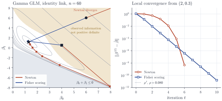
Left: contours of the log-likelihood of a gamma GLM with identity link, with Newton and Fisher scoring iterates from two starting points. Right: error of the iterates against iteration number on a log scale. — Figure 1. Left: contours of $\ell(\hat\beta) - \ell(\beta)$ (grey), the region where $J(\beta)$ is not positive definite (shaded), the region $\beta_0 + \beta_1 \le 0$, where the fitted mean at $x = 1$ would be nonpositive (bottom), and twelve iterations of each method from $(6, 6)$ (circles) and $(4, 0.5)$ (squares). Steps are halved only when they would leave the parameter space. Right: distance to $\hat\beta$ from the start $(2, 0.3)$; the dotted line decays like $\rho^t$, with $\rho$ the spectral radius of $I - \mathcal I(\hat\beta)^{-1} J(\hat\beta)$.

From $(6, 6)$ all fitted means are far above the data, $J$ is negative definite, and $\ell$ is locally convex. Newton’s method then heads for the stationary point of a convex quadratic, which lies further from the data, and the iterates run off to infinity. Fisher scoring reaches the maximizer to plotting accuracy after a single step. From $(4, 0.5)$ Newton’s method eventually converges after a long excursion toward the boundary of the parameter space. In the right panel, started near the maximizer, scoring converges linearly at exactly the rate $\rho \approx 0.08$ predicted by Proposition 2, while Newton’s method is slower at first and then overtakes it once the quadratic phase begins.

Remarks

A common hybrid starts with a few scoring iterations, which are robust, and finishes with Newton steps, which are fast; for canonical links there is nothing to choose. At convergence, $\mathcal I(\hat\beta)^{-1}$, with $\phi$ replaced by an estimate when it is unknown, is the usual model-based covariance, so scoring delivers standard errors as a by-product; when the observed and expected information differ, the observed version $J(\hat\beta)^{-1}$ is often preferred for inference.

Neither method can find a maximizer that does not exist. In logistic regression with completely separated data the likelihood increases along a ray to infinity; IRLS then produces coefficients that grow without bound and fitted probabilities approaching $0$ and $1$, and a diverging iteration of this kind signals that the maximum likelihood estimate does not exist.

The scoring method is due to Fisher, and its use for the whole class of generalized linear models to J. A. Nelder and R. W. M. Wedderburn, “Generalized linear models”, Journal of the Royal Statistical Society, Series A (1972). McCullagh and Nelder, Generalized Linear Models, treat the algorithm in detail, and P. J. Green, “Iteratively reweighted least squares for maximum likelihood estimation, and some robust and resistant alternatives”, Journal of the Royal Statistical Society, Series B (1984), discusses it as a general device.