Inducing points as variational parameters: a lower bound for sparse Gaussian processes
The classical inducing-point approximations (subset of regressors, DTC, FITC) change the Gaussian process prior and then do exact inference in the modified model. When the inducing inputs \(Z\) and the kernel hyperparameters are chosen by maximizing the marginal likelihood of the modified model, nothing ties the result to the model we actually wanted to fit. Titsias (Variational learning of inducing variables in sparse Gaussian processes, AISTATS 2009) proposed the opposite order: keep the exact model and approximate its posterior. The inducing values then define a variational family, the inducing inputs index that family, and the objective is a lower bound on the exact log marginal likelihood.
The notation follows the companion note on inducing points: \(f \sim \mathcal{GP}(0, k)\), training inputs \(X\) with \(f = f(X) \in \R^n\), \(y = f + \varepsilon\) with \(\varepsilon \sim \mathcal N(0, \sigma^2 I)\), inducing values \(u = f(Z) \in \R^m\) with \(K_{uu}\) invertible, \(A = K_{fu}K_{uu}^{-1}\) and \(Q_{ff} = K_{fu}K_{uu}^{-1}K_{uf}\).
Augmenting without changing the model
For any \(Z\), the joint law of \((y, f, u)\) is \(p(y\mid f)\,p(f\mid u)\,p(u)\) where \(p(f\mid u) = \mathcal N(Au, K_{ff} - Q_{ff})\). Integrating out \(u\) returns the original model. In particular the evidence \(p(y)\) and the posterior of \(f\) do not depend on \(Z\), so \(Z\) is not a model parameter. Titsias’s variational family keeps the prior conditional of \(f\) given \(u\) and frees only the distribution of \(u\):
\[q(f, u) = p(f\mid u)\, q(u).\]The conditional \(p(f\mid u)\) may be degenerate (for instance when an inducing input coincides with a training input), so it is cleaner to argue with Radon–Nikodym derivatives than with densities. Both \(q(f,u)\) and the exact posterior \(p(f, u\mid y) \propto p(y\mid f)\, p(f\mid u)\, p(u)\) share the conditional kernel \(p(f\mid u)\), and therefore
\[\log \frac{\dd q(f,u)}{\dd p(f,u\mid y)} = \log\frac{q(u)}{p(u)} - \log p(y\mid f) + \log p(y)\]whenever \(q(u)\) has a density with respect to \(p(u)\). The intractable conditional has cancelled.
Proposition 1. Let \(q(u)\) be a density with finite second moments and \(\mathrm{KL}(q(u)\Vert p(u)) < \infty\). Then \(\log p(y) = \mathcal L(q) + \mathrm{KL}\bigl(q(f,u)\Vert p(f,u\mid y)\bigr)\), where
\[\mathcal L(q) = \E_{q(u)}\bigl[\log \mathcal N(y\mid Au, \sigma^2 I)\bigr] - \frac{1}{2\sigma^2}\tr(K_{ff} - Q_{ff}) - \mathrm{KL}\bigl(q(u)\Vert p(u)\bigr).\]Proof. Taking expectations under \(q(f,u)\) in the display above gives \(\mathrm{KL}(q(f,u)\Vert p(f,u\mid y)) = \mathrm{KL}(q(u)\Vert p(u)) - \E_q \log p(y\mid f) + \log p(y)\). It remains to compute \(\E_q\log p(y\mid f)\). Given \(u\), \(f\) has mean \(Au\) and covariance \(K_{ff} - Q_{ff}\), so
\[\E\bigl[\norm{y - f}^2 \bigm\vert u\bigr] = \norm{y - Au}^2 + \tr(K_{ff} - Q_{ff}),\]and since \(\log p(y\mid f) = -\tfrac n2 \log(2\pi\sigma^2) - \norm{y-f}^2/(2\sigma^2)\), we get \(\E\bigl[\log p(y\mid f)\bigm\vert u\bigr] = \log\mathcal N(y\mid Au, \sigma^2 I) - \tr(K_{ff} - Q_{ff})/(2\sigma^2)\). Averaging over \(q(u)\), which is legitimate because \(q(u)\) has finite second moments, gives the claim.
The collapsed bound
The bound depends on \(q(u)\) only through a Gaussian log-likelihood term and a Kullback–Leibler penalty, and this combination has an explicit maximizer.
Proposition 2. Over all \(q(u)\) as in Proposition 1,
\[\mathcal L^\ast(Z) := \max_{q} \mathcal L(q) = \log\mathcal N\bigl(y\mid 0,\, Q_{ff} + \sigma^2 I\bigr) - \frac{1}{2\sigma^2}\tr\bigl(K_{ff} - Q_{ff}\bigr),\]attained uniquely at \(q^\ast(u) \propto \mathcal N(y\mid Au, \sigma^2 I)\, p(u)\), that is, \(q^\ast = \mathcal N\bigl(\sigma^{-2}K_{uu}\Sigma K_{uf}y,\; K_{uu}\Sigma K_{uu}\bigr)\) with \(\Sigma = (K_{uu} + \sigma^{-2}K_{uf}K_{fu})^{-1}\).
Proof. Write \(g(u) = \log\mathcal N(y\mid Au, \sigma^2 I)\) and \(Z_g = \int e^{g}\, \dd p(u)\). With \(q^\ast = e^{g}p/Z_g\), a direct expansion gives
\[\E_q g - \mathrm{KL}(q\Vert p) = \log Z_g - \mathrm{KL}(q\Vert q^\ast),\]which is maximized exactly when \(q = q^\ast\). The normalizer is the marginal density of \(y\) in the linear model \(y = Au + e\), \(u \sim \mathcal N(0, K_{uu})\), \(e \sim \mathcal N(0, \sigma^2 I)\), namely \(Z_g = \mathcal N(y\mid 0, AK_{uu}A^\top + \sigma^2 I) = \mathcal N(y\mid 0, Q_{ff} + \sigma^2 I)\). The form of \(q^\ast\) is the conjugate Gaussian update for the same linear model.
The optimal \(q^\ast(u)\) coincides with the posterior of \(u\) under DTC, and the predictive distribution \(\int p(f_\ast\mid u)\, q^\ast(u)\, \dd u\) is the DTC predictive distribution. The variational method therefore does not produce new predictive equations. What it changes is the objective. The first term of \(\mathcal L^\ast\) is the DTC marginal likelihood; the second,
\[\frac{1}{2\sigma^2}\tr(K_{ff} - Q_{ff}) = \frac{1}{2\sigma^2}\sum_{i=1}^n \Var\bigl(f(x_i)\bigm\vert u\bigr),\]penalizes inducing sets that leave the latent function at the training inputs poorly determined. It is what makes \(\mathcal L^\ast\) a bound on the exact evidence. Both terms cost \(O(nm^2)\): the log-density through the Woodbury identity and the matrix determinant lemma, the trace through the diagonal of \(Q_{ff}\).
Properties of the bound
Proposition 3.
- \(\mathcal L^\ast(Z) \le \log p(y)\), and the gap equals \(\mathrm{KL}\bigl(p(f\mid u)q^\ast(u)\Vert p(f,u\mid y)\bigr)\).
- If \(Z \subseteq Z'\), then \(\mathcal L^\ast(Z) \le \mathcal L^\ast(Z')\).
- If every training input belongs to \(Z\), then \(\mathcal L^\ast(Z) = \log p(y)\).
Proof. Part 1 is Proposition 1 at \(q = q^\ast\). For part 2 write \(u' = (u, v)\) with \(v\) the values at \(Z' \setminus Z\), and take any \(q(u)\) admissible for \(Z\). The distribution \(q'(u, v) = q(u)\,p(v\mid u)\) is admissible for \(Z'\), and the corresponding variational distribution \(p(f\mid u, v)\,q'(u,v) = p(f, v\mid u)\,q(u)\) has the same marginal law of \(f\) as \(p(f\mid u)\, q(u)\). Hence the expected log-likelihood terms agree, and \(\mathrm{KL}(q'\Vert p(u,v)) = \mathrm{KL}\bigl(q(u)p(v\mid u)\Vert p(u)p(v\mid u)\bigr) = \mathrm{KL}(q\Vert p(u))\). So every value of the bound attainable with \(Z\) is attainable with \(Z'\). For part 3, if \(X \subseteq Z\) then \(f\) is a coordinate projection of \(u\), so \(\Var(f(x_i)\mid u) = 0\) and \(Q_{ff} = K_{ff}\); the trace vanishes and the first term is \(\log\mathcal N(y\mid 0, K_{ff} + \sigma^2 I) = \log p(y)\).
Part 2 is the property that the approximate-model objectives lack: since the bound can only increase when inducing inputs are added, and never exceeds the exact evidence, optimizing \(Z\) cannot overfit in the sense of moving away from the exact model. The worst that can happen is that extra inducing inputs are wasted.
Figure 1 tracks the bound along a nested sequence of inducing sets, obtained by adding training inputs in random order. The bound increases monotonically, as part 2 requires; the trace penalty accounts for most of the gap when \(m\) is small and for about half of it once the gap is small. The DTC marginal likelihood lies above the bound by exactly the trace term; it is not itself a bound on \(\log p(y)\) in general, and with few inducing inputs it is considerably more optimistic about how well the approximation explains the data.
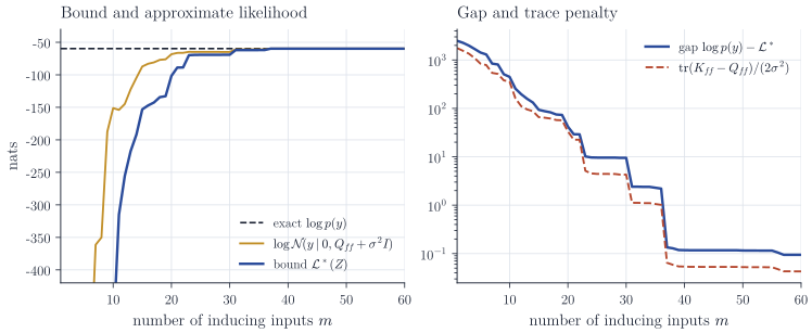
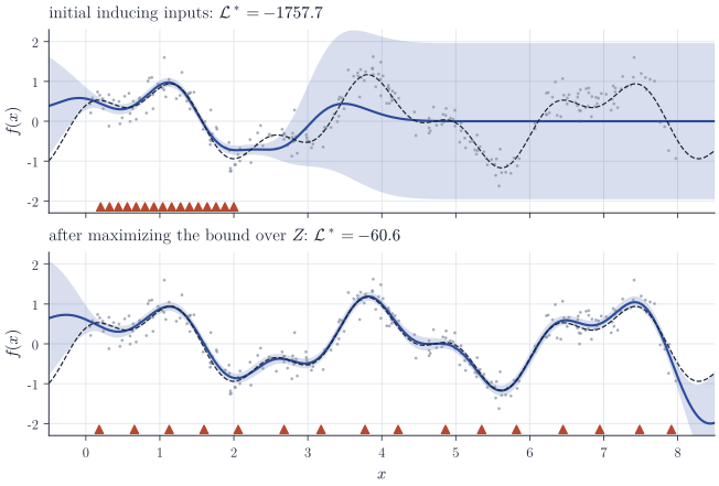
Figure 2 shows the effect of maximizing \(\mathcal L^\ast\) over \(Z\) numerically, with the hyperparameters fixed. Sixteen inducing inputs start clustered on \([0.2, 2]\), where the approximation is good locally and reverts to the prior elsewhere; the starting value of the bound is \(-1757.7\) nats. After optimization they spread over the data and the bound is \(-60.6\), against \(-61.6\) for sixteen evenly spaced inputs and \(-59.7\) for the exact evidence. The objective is not concave in \(Z\): in a run of L-BFGS without the box constraint \(Z \subset [0, 8]\), the optimizer pushed two inducing inputs far outside the data (to about \(18.6\) and \(21.7\)), where they have no effect, and stopped at the worse value \(-64.6\).
Hyperparameters
The kernel hyperparameters \(\theta\) (here \(\ell, \sigma_f, \sigma\)) are usually optimized jointly with \(Z\). Because \(\mathcal L^\ast(Z, \theta) \le \log p(y\mid\theta)\) for every \(\theta\), this maximizes a lower bound on the type-II likelihood, and the gap varies with \(\theta\). The maximizer is therefore biased towards hyperparameters for which the sparse approximation is accurate. One visible consequence is in the noise variance: the trace penalty is divided by \(\sigma^2\), so a larger noise variance makes the penalty smaller, and the bound tends to favour noise estimates that are too large when \(m\) is too small to explain the data. This bias goes in the safe direction (underfitting rather than overfitting), and it disappears as the gap closes.
Remarks
Proposition 2 eliminated \(q(u)\) analytically. Keeping \(q(u) = \mathcal N(\mu, S)\) explicit instead gives the bound of Proposition 1, which is a sum over observations plus one Kullback–Leibler term; Hensman, Fusi and Lawrence (Gaussian processes for big data, UAI 2013) optimize it by stochastic variational inference with minibatches, which removes the \(O(n)\) cost per step and also allows non-Gaussian likelihoods. How quickly \(m\) must grow with \(n\) for the gap to vanish depends on the eigenvalue decay of the kernel operator; Burt, Rasmussen and van der Wilk (Rates of convergence for sparse variational Gaussian process regression, ICML 2019) give bounds of this kind.