Inducing points: Gaussian process prediction through a low-rank summary
Gaussian process regression with \(n\) observations requires a Cholesky factorization of the \(n \times n\) matrix \(K_{ff} + \sigma^2 I\), which costs \(O(n^3)\) time and \(O(n^2)\) memory. For a smooth kernel this matrix is also numerically close to low rank: once inputs are much denser than the length-scale, neighbouring function values carry nearly the same information. Inducing-point methods exploit this by choosing \(m \ll n\) inputs \(Z = (z_1, \dots, z_m)\) and letting the vector \(u = (f(z_1), \dots, f(z_m))\) act as a summary of the function. The three classical approximations of this kind all follow from one decomposition of the prior; the presentation below follows the unifying treatment of Quiñonero-Candela and Rasmussen (A unifying view of sparse approximate Gaussian process regression, Journal of Machine Learning Research, 2005).
Notation: \(f \sim \mathcal{GP}(0, k)\); training inputs \(X = (x_1, \dots, x_n)\) with \(f = f(X)\) and responses \(y = f + \varepsilon\), \(\varepsilon \sim \mathcal N(0, \sigma^2 I)\) independent of \(f\); \(f_\ast = f(x_\ast)\) at a test input. Kernel matrices are written \(K_{ab} = k(a, b)\), for instance \(K_{fu} = k(X, Z)\) and \(K_{uu} = k(Z, Z)\), the latter assumed invertible.
What the inducing values know
By the Gaussian conditioning lemma applied to \((f(\cdot), u)\), conditionally on \(u\) the process is again Gaussian,
\[f(\cdot) \mid u \sim \mathcal{GP}\bigl( k(\cdot, Z) K_{uu}^{-1} u,\; k - q \bigr), \qquad q(x, x') = k(x, Z) K_{uu}^{-1} k(Z, x').\]The kernel \(q\) is the Nyström approximation of \(k\) based on \(Z\), and we write \(Q_{ab} = K_{au}K_{uu}^{-1}K_{ub}\) for its matrices. Since \(\E[f(\cdot) \mid u] = k(\cdot, Z)K_{uu}^{-1}u\), we have \(q(x, x') = \Cov\bigl(\E[f(x)\mid u], \E[f(x')\mid u]\bigr)\), and the law of total covariance splits the prior into the part explained by \(u\) and the part that is not:
\[k(x, x') = q(x, x') + \E\bigl[\Cov(f(x), f(x') \mid u)\bigr].\]Proposition 1. For any finite set of inputs, \(0 \preceq Q \preceq K\) in the positive semidefinite order. If \(Z \subseteq Z'\) and \(Q, Q'\) are the corresponding Nyström matrices, then \(Q \preceq Q'\).
Proof. Fix inputs \(t_1, \dots, t_p\) and let \(F = (f(t_1), \dots, f(t_p))\). Then \(Q = \Cov(\E[F\mid u])\) and \(K - Q = \E \Cov(F\mid u)\) are covariance matrices, hence positive semidefinite. If \(Z \subseteq Z'\), then \(u\) is a function of \(u'\), so \(\E[F\mid u] = \E\bigl[\E[F\mid u'] \bigm\vert u\bigr]\) and, by the law of total covariance applied to \(G = \E[F\mid u']\),
\[Q' = \Cov(G) = \Cov(\E[G\mid u]) + \E\Cov(G\mid u) \succeq \Cov(\E[F\mid u]) = Q .\]Adding inducing inputs can therefore only enlarge the low-rank part, and \(\tr(K_{ff} - Q_{ff})\), the total conditional variance of the training values given \(u\), measures what the summary misses.
Three approximate priors
The joint prior of training and test values can be written exactly as \(p(f, f_\ast) = \int p(f\mid u)\, p(f_\ast\mid u)\, p(u)\, \dd u\) only if \(f\) and \(f_\ast\) are conditionally independent given \(u\), which is false in general; this conditional independence is the first approximation shared by all methods below. They then differ in what they use for the training conditional \(p(f \mid u) = \mathcal N(K_{fu}K_{uu}^{-1}u,\, K_{ff} - Q_{ff})\) and the test conditional \(p(f_\ast\mid u) = \mathcal N(K_{\ast u}K_{uu}^{-1}u,\, k_{\ast\ast} - q_{\ast\ast})\):
- Subset of regressors (SoR): both conditionals are replaced by their means, so \(f(\cdot) = k(\cdot, Z)K_{uu}^{-1}u\). This is a Bayesian linear model with the \(m\) basis functions \(k(\cdot, z_j)\) and coefficients \(w = K_{uu}^{-1}u \sim \mathcal N(0, K_{uu}^{-1})\), that is, a Gaussian process with the degenerate kernel \(q\).
- Deterministic training conditional (DTC): the training conditional is replaced by its mean, the test conditional is kept exact.
- Fully independent training conditional (FITC): the training conditional keeps its exact marginal variances but drops correlations, \(\mathcal N\bigl(K_{fu}K_{uu}^{-1}u,\, \diag(K_{ff} - Q_{ff})\bigr)\); the test conditional is exact. This approximation was introduced by Snelson and Ghahramani (Sparse Gaussian processes using pseudo-inputs, NIPS 2005).
In all three cases the model for the responses is \(y \mid u \sim \mathcal N(K_{fu}K_{uu}^{-1}u,\, \Lambda)\) with \(\Lambda = \sigma^2 I\) for SoR and DTC and \(\Lambda = \diag(K_{ff} - Q_{ff}) + \sigma^2 I\) for FITC, a diagonal matrix in every case.
Proposition 2. Let \(\Sigma = \bigl(K_{uu} + K_{uf}\Lambda^{-1}K_{fu}\bigr)^{-1}\). Under each approximate prior, \(u \mid y \sim \mathcal N\bigl(K_{uu}\Sigma K_{uf}\Lambda^{-1}y,\; K_{uu}\Sigma K_{uu}\bigr)\), and the predictive distribution of \(f_\ast\) is Gaussian with mean
\[\mu_\ast = K_{\ast u}\, \Sigma\, K_{uf}\Lambda^{-1} y\]and variance \(K_{\ast u}\Sigma K_{u\ast}\) for SoR, and \(k_{\ast\ast} - q_{\ast\ast} + K_{\ast u}\Sigma K_{u\ast}\) for DTC and FITC.
Proof. With \(A = K_{fu}K_{uu}^{-1}\), the model is \(u \sim \mathcal N(0, K_{uu})\) and \(y\mid u \sim \mathcal N(Au, \Lambda)\). Completing the square in \(\log p(u) + \log p(y\mid u)\) gives a Gaussian posterior with precision and mean
\[P = K_{uu}^{-1} + A^\top\Lambda^{-1}A = K_{uu}^{-1}\bigl(K_{uu} + K_{uf}\Lambda^{-1}K_{fu}\bigr)K_{uu}^{-1} = K_{uu}^{-1}\Sigma^{-1}K_{uu}^{-1}, \qquad P^{-1}A^\top\Lambda^{-1}y,\]so the posterior covariance is \(K_{uu}\Sigma K_{uu}\) and the mean is \(K_{uu}\Sigma K_{uu}K_{uu}^{-1}K_{uf}\Lambda^{-1}y = K_{uu}\Sigma K_{uf}\Lambda^{-1}y\). In every method \(f_\ast \mid u\) has mean \(K_{\ast u}K_{uu}^{-1}u\) and is conditionally independent of \(y\) given \(u\), so \(\E[f_\ast\mid y] = K_{\ast u}K_{uu}^{-1}\E[u\mid y] = \mu_\ast\) and
\[\Var(f_\ast\mid y) = \Var(f_\ast\mid u) + K_{\ast u}K_{uu}^{-1}\Cov(u\mid y)K_{uu}^{-1}K_{u\ast},\]where the second term equals \(K_{\ast u}\Sigma K_{u\ast}\) and the first is \(0\) for SoR and \(k_{\ast\ast} - q_{\ast\ast}\) for DTC and FITC.
Only \(m \times m\) matrices are inverted. Forming \(K_{uf}\Lambda^{-1}K_{fu}\) costs \(O(nm^2)\), its Cholesky factorization \(O(m^3)\), and afterwards a predictive mean costs \(O(m)\) and a variance \(O(m^2)\). The mean is a combination of the \(m\) functions \(k(\cdot, z_j)\) rather than the \(n\) functions \(k(\cdot, x_i)\) of the exact posterior. SoR and DTC have the same mean and differ only in the variance; FITC changes the mean as well, because its \(\Lambda\) down-weights observations whose function values are poorly explained by \(u\). When \(Z = X\) and \(K_{ff}\) is invertible, so that \(Q_{ff} = K_{ff}\), a short calculation with \(\Sigma = (K_{ff} + \sigma^{-2}K_{ff}^2)^{-1}\) shows that DTC and FITC reproduce the exact posterior, while SoR still uses \(q_{\ast\ast}\) in place of \(k_{\ast\ast}\) at test inputs.
Where the approximations differ
The difference in variance is the visible one. Far from all inducing inputs, \(K_{\ast u} \to 0\) for a kernel that decays with distance, so the SoR predictive variance tends to zero: the approximate prior has no variance there to begin with, since \(q(x,x) \le k(x,x)\) and \(q(x,x) \to 0\). SoR is thus confidently wrong exactly where data are absent. DTC and FITC add back \(k_{\ast\ast} - q_{\ast\ast}\) and revert to the prior variance away from \(Z\), as the exact posterior does.
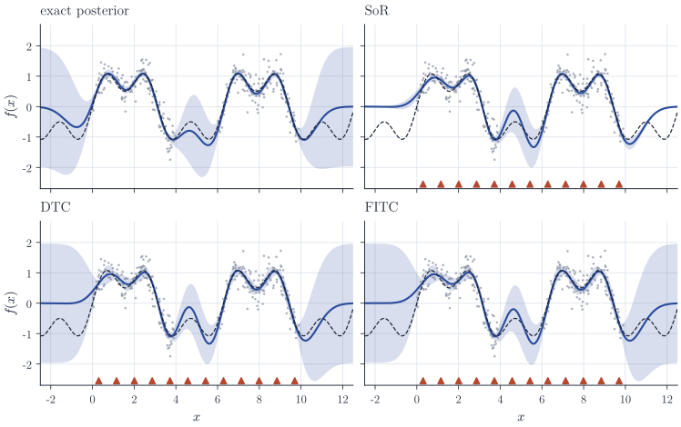
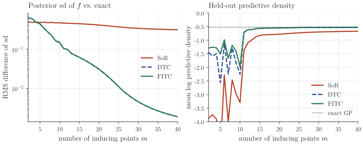
Figure 2 measures this as \(m\) grows with the inducing inputs evenly spaced on the same interval. For DTC and FITC the posterior standard deviation converges to the exact one; for SoR it does not, because no inducing input lies in the extrapolation region and the collapse there persists. The held-out log predictive density shows the same ordering. With too few inducing inputs, here fewer than about one per length-scale, every method fails: the mean itself is wrong, and the variance cannot compensate.
Choosing the inducing inputs
The inducing inputs can be a random subset of the data, a grid, or cluster centres. They can also be treated as parameters and optimized together with the kernel hyperparameters by maximizing the marginal likelihood of the approximate model, \(\log \mathcal N(y \mid 0, Q_{ff} + \Lambda)\), whose determinant and inverse are again computable in \(O(nm^2)\) by the matrix determinant lemma and the Woodbury identity. This is the approach of Snelson and Ghahramani for FITC. The difficulty is that this objective is the marginal likelihood of the approximate model, not of the Gaussian process being approximated: improving it can move the approximate model away from the exact Gaussian process, and FITC in particular is known to underestimate the noise variance when \(Z\) is optimized; Bauer, van der Wilk and Rasmussen (Understanding probabilistic sparse Gaussian process approximations, NeurIPS 2016) analyse this behaviour.
Remarks
Proposition 2 shows that all three methods are Bayesian linear models in \(m\) coefficients that differ only in their noise model and in whether the test conditional variance \(k_{\ast\ast} - q_{\ast\ast}\) is restored. A different way to choose \(Z\) keeps the exact model and introduces a Gaussian variational distribution for \(u\); the inducing inputs and hyperparameters are then chosen by maximizing a lower bound on the exact log marginal likelihood, so that improving the objective cannot move the model away from the exact Gaussian process. This is the variational approach of Titsias (Variational learning of inducing variables in sparse Gaussian processes, AISTATS 2009), whose predictive mean and variance have the DTC form, and whose bound differs from the DTC marginal likelihood by the penalty \(-\tr(K_{ff} - Q_{ff})/(2\sigma^2)\). Chapter 8 of Rasmussen and Williams, Gaussian Processes for Machine Learning, surveys these and other approximations.