Priors with infinite mass: when an improper prior still gives a proper posterior
A prior that spreads equal weight over the whole real line cannot be a probability distribution: Lebesgue measure on \(\R\) has infinite mass. Such priors are nonetheless used constantly, as defaults for location parameters, as \(1/\sigma\) for scale parameters, and as the reference or Jeffreys priors of objective Bayesian analysis. Bayes’ formula still makes sense for them provided one quantity, the marginal density of the data, is finite. When it is, the resulting posterior is the limit of posteriors under proper truncations of the prior; when it is not, there is no posterior at all, and this happens in models used every day.
The formal posterior
Let \(\Theta \subseteq \R^d\) be a Borel set, and let \(\{f(\cdot \mid \theta) : \theta \in \Theta\}\) be densities on a sample space \(\mathcal X\) with respect to a \(\sigma\)-finite measure, such that \((x, \theta) \mapsto f(x \mid \theta)\) is jointly measurable. A prior is a measurable function \(\pi : \Theta \to [0, \infty)\), read as a density of the measure \(\Pi(A) = \int_A \pi(\theta) \, \dd\theta\). The prior is improper if \(\Pi(\Theta) = \infty\). Since \(\pi\) takes finite values, \(\Pi\) is automatically \(\sigma\)-finite.
For an observation \(x\) define the marginal
\[m(x) = \int_\Theta f(x \mid \theta) \, \pi(\theta) \, \dd\theta \in [0, \infty].\]When \(0 < m(x) < \infty\), the formal posterior
\[\pi(\theta \mid x) = \frac{f(x \mid \theta) \, \pi(\theta)}{m(x)}\]is a probability density on \(\Theta\). When \(m(x) = \infty\) the expression has no meaning: \(f(x \mid \theta)\pi(\theta)\) is still a nonnegative function of \(\theta\), but no constant turns it into a probability density. A sampler applied to it does not approximate any distribution. The posterior is then called improper.
Two features distinguish this from the proper case. First, \(\pi\) and \(c\pi\) give the same formal posterior for every \(c > 0\), while \(m(x)\) is multiplied by \(c\). Quantities built from \(m(x)\) itself, such as Bayes factors, are therefore undefined under improper priors. Second, whether \(m(x) < \infty\) can depend on the observed \(x\). For a proper prior, Tonelli’s theorem gives \(\int m(x) \, \dd x = 1\), so \(m(x) < \infty\) for almost every \(x\). Nothing of the kind holds for a prior of infinite mass.
Two cases that work
Location. Let \(X_1, \dots, X_n\) be independent \(N(\theta, \sigma^2)\) with \(\sigma\) known and \(\pi(\theta) = 1\) on \(\R\). Expanding the square around \(\bar x\),
\[\prod_{i=1}^n f(x_i \mid \theta) = (2\pi\sigma^2)^{-n/2} \exp\Bigl(-\frac{\sum_i (x_i - \bar x)^2}{2\sigma^2}\Bigr) \exp\Bigl(-\frac{n(\theta - \bar x)^2}{2\sigma^2}\Bigr),\]whose integral over \(\theta\) is finite for every sample. The formal posterior is \(N(\bar x, \sigma^2/n)\), and the equal-tailed 95% credible interval coincides with the classical confidence interval \(\bar x \pm 1.96 \, \sigma/\sqrt n\).
Scale. Let \(X_1, \dots, X_n\) be independent \(N(0, \sigma^2)\) and \(\pi(\sigma) = 1/\sigma\) on \((0, \infty)\). With \(s = \sum_i x_i^2\) the unnormalized posterior is \(\sigma^{-n-1} e^{-s/(2\sigma^2)}\). The substitution \(u = s/(2\sigma^2)\) gives
\[\int_0^\infty \sigma^{-n-1} e^{-s/(2\sigma^2)} \, \dd\sigma = \tfrac12 \, (s/2)^{-n/2} \, \Gamma(n/2),\]finite whenever \(s > 0\), which holds with probability one. Both priors are invariant: Lebesgue measure under translations \(\theta \mapsto \theta + c\), and \(\dd\sigma/\sigma\) under rescalings \(\sigma \mapsto c\sigma\). They are the Haar measures of the translation and scale groups, and that invariance is the usual argument for them. No proper distribution on \(\R\) is translation invariant, so the argument forces improperness.
Improper priors as limits of proper ones
A natural way to justify a formal posterior is to approximate the improper prior by proper ones. When the marginal is finite, this works in the strongest sense one could ask for.
Proposition 1. Suppose \(0 < m(x) < \infty\). Let \(K_1 \subseteq K_2 \subseteq \cdots\) be Borel sets with \(\bigcup_j K_j = \Theta\) and \(0 < \Pi(K_j) < \infty\), and let \(\pi_j = \pi \, \mathbf 1_{K_j} / \Pi(K_j)\) be the restricted and normalized priors. Then for all large \(j\) the posterior \(\pi_j(\cdot \mid x)\) exists, and
\[\sup_{A} \Bigl\lvert \int_A \pi_j(\theta \mid x) \, \dd\theta - \int_A \pi(\theta \mid x) \, \dd\theta \Bigr\rvert = 1 - \frac{m_j(x)}{m(x)} \longrightarrow 0,\]where \(m_j(x) = \int_{K_j} f(x \mid \theta)\pi(\theta)\,\dd\theta\) and the supremum runs over Borel sets \(A \subseteq \Theta\).
Proof. The normalizing constant \(\Pi(K_j)\) cancels, so \(\pi_j(\theta \mid x) = f(x \mid \theta)\pi(\theta)\mathbf 1_{K_j}(\theta)/m_j(x)\). By monotone convergence \(m_j(x) \uparrow m(x)\), so \(m_j(x) > 0\) for large \(j\). On \(K_j\) the difference \(\pi_j(\theta \mid x) - \pi(\theta \mid x)\) equals \(f(x \mid \theta)\pi(\theta)\bigl(1/m_j(x) - 1/m(x)\bigr) \ge 0\), and off \(K_j\) it equals \(-\pi(\theta \mid x)\). The supremum of \(\int_A (\pi_j - \pi)(\theta \mid x)\,\dd\theta\) is attained at \(A = K_j\) and equals
\[\frac{m_j(x)}{m_j(x)} - \frac{m_j(x)}{m(x)} = 1 - \frac{m_j(x)}{m(x)} .\]Since both densities integrate to one, the supremum of the negative part is the same number, which tends to zero.
The finiteness of \(m(x)\) carries the whole argument. When \(m(x) = \infty\) the ratio \(m_j(x)/m(x)\) is meaningless, and the truncated posteriors typically lose mass to the boundary of \(\Theta\) or to infinity instead of converging to a distribution. The proposition also says nothing about the frequentist or decision-theoretic quality of the limit. A flat prior on \(\R^p\) for a normal mean gives posterior mean \(\bar x\), which is inadmissible under squared error loss when \(p \ge 3\), by Stein’s result.
A prior that fails for some samples
Let \(X \sim \mathrm{Binomial}(n, \theta)\) and take Haldane’s prior \(\pi(\theta) = \theta^{-1}(1-\theta)^{-1}\) on \((0, 1)\), the formal limit of \(\mathrm{Beta}(\varepsilon, \varepsilon)\) as \(\varepsilon \downarrow 0\). The unnormalized posterior is \(\theta^{x-1}(1-\theta)^{n-x-1}\), which is integrable if and only if \(x \ge 1\) and \(n - x \ge 1\). For \(1 \le x \le n-1\) the posterior is \(\mathrm{Beta}(x, n - x)\) with mean \(x/n\). For \(x = 0\) the integrand behaves like \(\theta^{-1}\) near zero, so \(m(0) = \infty\).
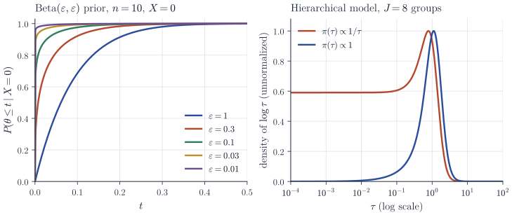
By symmetry \(m(n) = \infty\) as well, so the posterior fails to exist with probability \((1-\theta)^n + \theta^n\), which is far from negligible for rare events. Proper approximations show where the mass goes. Under \(\mathrm{Beta}(\varepsilon, \varepsilon)\) and \(x = 0\) the posterior is \(\mathrm{Beta}(\varepsilon, n + \varepsilon)\), with mean \(\varepsilon/(n + 2\varepsilon)\). By Markov’s inequality the posterior probability of \(\{\theta > t\}\) is at most \(\varepsilon/(t(n + 2\varepsilon))\) for each \(t > 0\), so the posteriors converge weakly to the point mass at \(\theta = 0\) (left panel of Figure 1). The limiting “posterior” asserts certainty that the event is impossible, after a finite number of trials.
Variance components in hierarchical models
The most consequential failure occurs in hierarchical models, where the \(1/\tau\) prior that the invariance argument suggests for a scale parameter gives no posterior at all. Consider \(J\) groups with
\[y_j \mid \theta_j \sim N(\theta_j, s_j^2), \qquad \theta_j \mid \mu, \tau \sim N(\mu, \tau^2), \qquad j = 1, \dots, J,\]independently, with known \(s_j > 0\), a flat prior on \(\mu \in \R\) and a prior \(\pi(\tau)\) on \(\tau \in (0, \infty)\). Integrating out each \(\theta_j\) gives \(y_j \mid \mu, \tau \sim N(\mu, s_j^2 + \tau^2)\). Write \(w_j = 1/(s_j^2 + \tau^2)\), \(W = \sum_j w_j\) and \(\hat\mu = W^{-1}\sum_j w_j y_j\). Integrating \(\mu\) against Lebesgue measure, again by completing the square,
\[\begin{equation} \begin{aligned} L(\tau) &:= \int_\R \prod_{j=1}^J N(y_j; \mu, s_j^2 + \tau^2) \, \dd\mu \\ &= (2\pi)^{-(J-1)/2} \, W^{-1/2} \prod_{j=1}^J w_j^{1/2} \exp\Bigl(-\frac12 \sum_{j=1}^J w_j (y_j - \hat\mu)^2\Bigr), \end{aligned} \label{eq:marg-tau} \end{equation}\]and the posterior of \(\tau\) is proportional to \(L(\tau)\pi(\tau)\), whenever this is integrable.
Proposition 2. Let \(J \ge 2\) and \(\pi(\tau) = \tau^{-a}\) with \(a \in \R\). For every data vector \(y\), the posterior of \(\tau\) is proper if and only if \(2 - J < a < 1\). In particular \(\pi(\tau) \propto 1/\tau\) never gives a proper posterior, and the flat prior \(\pi(\tau) \propto 1\) does so if and only if \(J \ge 3\).
Proof. Each \(w_j\) is continuous and positive on \([0, \infty)\), so \(W\) is continuous and positive, and \(\hat\mu\) and the exponent in \(\eqref{eq:marg-tau}\) are continuous. Hence \(L\) is continuous and strictly positive on \([0, \infty)\), with \(L(0) > 0\), and integrability of \(L(\tau)\tau^{-a}\) can only fail near \(0\) or near \(\infty\).
Near zero, \(L(\tau)\tau^{-a}\) is bounded above and below by positive multiples of \(\tau^{-a}\), which is integrable on \((0, 1)\) if and only if \(a < 1\).
Near infinity, \(\tau^2 w_j \to 1\) for every \(j\), so \(\prod_j w_j^{1/2} \sim \tau^{-J}\) and \(W^{-1/2} \sim \tau/\sqrt J\). For the exponent, \(\hat\mu\) minimizes \(c \mapsto \sum_j w_j (y_j - c)^2\), so
\[0 \le \sum_j w_j (y_j - \hat\mu)^2 \le \sum_j w_j (y_j - \bar y)^2 \le \tau^{-2} \sum_j (y_j - \bar y)^2 \to 0 .\]Therefore \(L(\tau) \sim (2\pi)^{-(J-1)/2} J^{-1/2} \, \tau^{-(J-1)}\) as \(\tau \to \infty\), and \(\int_1^\infty \tau^{-(J-1) - a} \, \dd\tau < \infty\) if and only if \(J - 1 + a > 1\).
The failure at zero has a simple explanation. As \(\tau \to 0\) the model reduces to complete pooling, \(\theta_j = \mu\) for all \(j\), which has positive likelihood for any data. The marginal likelihood therefore does not vanish at \(\tau = 0\), while \(1/\tau\) places infinite mass on every interval \((0, \delta)\). On the scale of \(\log \tau\), the prior \(1/\tau\) is flat on \(\R\) and the likelihood tends to a positive constant as \(\log\tau \to -\infty\), which is what the right panel of Figure 1 shows. Data cannot rescue the posterior: the conclusion holds for every \(y\).
The danger in practice is that nothing visibly breaks. A Gibbs sampler for this model has well-defined full conditionals, each of them proper, and it will produce output that looks like any other; the chain can drift towards \(\tau = 0\) and linger there, often slowly enough that a short run appears stable. Hobert and Casella (1996, Journal of the American Statistical Association) analysed this phenomenon for Gibbs samplers in hierarchical linear mixed models. Propriety of a joint posterior must be checked analytically, since it cannot be read off the full conditionals.
Remarks
Several other difficulties are specific to improper priors. Dawid, Stone and Zidek (1973, Journal of the Royal Statistical Society, Series B) constructed marginalization paradoxes, in which two apparently valid ways of computing the posterior of a function of the parameter disagree under an improper prior; no such inconsistency can arise with proper priors. Because improper priors are defined only up to a constant, Bayes factors and posterior model probabilities computed with them are arbitrary, which is one reason that Lindley’s paradox cannot be avoided by “letting the prior variance go to infinity”. For variance parameters in hierarchical models, Gelman (2006, Bayesian Analysis) discusses proper weakly informative alternatives such as half-\(t\) and half-Cauchy priors on \(\tau\). Kass and Wasserman (1996, Journal of the American Statistical Association) survey formal rules for choosing priors, including the role of improper ones, and Berger, Statistical Decision Theory and Bayesian Analysis, treats improper priors from the decision-theoretic side.