Thin shells and orthogonal directions: where volume and probability live in high dimensions
Pictures drawn in the plane are the main source of geometric intuition, and in high dimension several of them mislead. The centre of a ball contains almost none of its volume; the most likely point of a Gaussian distribution is a point near which the distribution almost never lands; two random directions are almost always nearly perpendicular. Each of these statements is elementary, and each has consequences for statistics and computation: for Monte Carlo methods, for nearest-neighbour methods, and for the difference between the mode of a posterior and where its mass is. Most of them follow from one concentration inequality for the length of a Gaussian vector.
Throughout, \(\norm{\cdot}\) is the Euclidean norm on \(\R^d\), \(B_d = \{x : \norm x \le 1\}\) is the unit ball and \(\lambda_d\) is Lebesgue measure.
Volume concentrates at the boundary
Scaling by \(r > 0\) multiplies \(d\)-dimensional volume by \(r^d\), so the fraction of \(B_d\) within distance \(\varepsilon\) of its boundary is
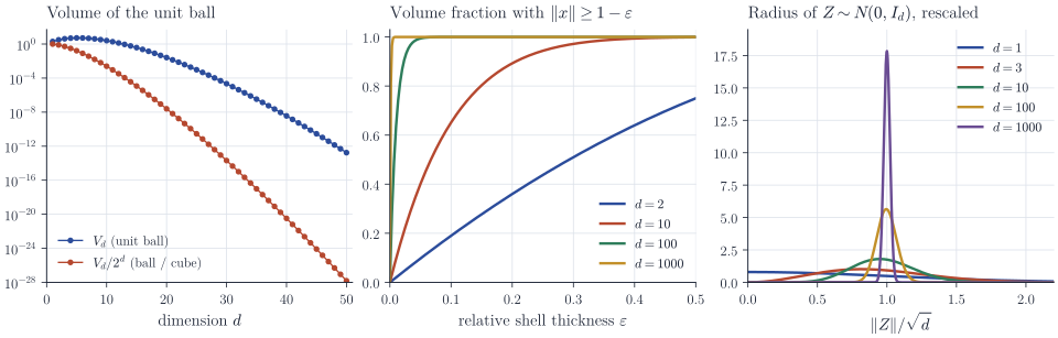
\[\frac{\lambda_d(B_d) - \lambda_d\bigl((1-\varepsilon)B_d\bigr)}{\lambda_d(B_d)} = 1 - (1-\varepsilon)^d \ge 1 - e^{-\varepsilon d}.\]For \(d = 1000\), the outer shell of relative thickness \(0.01\) contains all but \(e^{-10} \approx 5\times10^{-5}\) of the volume. Nothing here is special to balls: for any measurable set \(S\) of finite positive volume that is star-shaped about the origin, \((1-\varepsilon)S \subseteq S\) and the fraction of \(S\) lying outside \((1-\varepsilon)S\) is again \(1 - (1-\varepsilon)^d\), since the computation only uses scaling.
The volume of the ball itself also behaves unexpectedly. Write \(V_d = \lambda_d(B_d)\).
Proposition 1. \(V_d = \pi^{d/2}/\Gamma(d/2 + 1)\). In particular \(V_d \to 0\), and faster than any exponential: \(V_d^{1/d}\sqrt{d} \to \sqrt{2\pi e}\).
Proof. Compute \(I = \int_{\R^d}e^{-\norm x^2}\,\dd x\) in two ways. By Fubini it equals \(\bigl(\int_\R e^{-t^2}\dd t\bigr)^d = \pi^{d/2}\). On the other hand, the layer-cake formula \(\int g = \int_0^\infty\lambda_d(g > s)\,\dd s\) for the nonnegative function \(g(x) = e^{-\norm x^2}\) gives, with \(\{g > s\} = \sqrt{\log(1/s)}\,B_d\) for \(0 < s < 1\) and the substitution \(s = e^{-r^2}\),
\[I = \int_0^1 V_d\,\bigl(\log(1/s)\bigr)^{d/2}\,\dd s = V_d\int_0^\infty r^d\cdot 2re^{-r^2}\,\dd r = V_d\,\Gamma\bigl(\tfrac d2 + 1\bigr),\]where the last step substitutes \(u = r^2\). The asymptotics follow from Stirling’s formula, \(\log\Gamma(d/2+1) = \tfrac d2\log\tfrac d{2e} + O(\log d)\).
The volume increases up to \(d = 5\), where \(V_5 \approx 5.26\), and then decreases to zero. Compared with the cube \([-1,1]^d\) that circumscribes it, the ball is negligible: \(V_d/2^d\) is about \(0.0025\) for \(d = 10\) and below \(10^{-27}\) for \(d = 50\) (Figure 1, left). Almost all of the cube lies outside the inscribed ball: a uniform point of the cube has \(\E\norm X^2 = d/3\), and Hoeffding’s inequality applied to the independent bounded variables \(X_i^2\) shows that its distance from the centre is \(\sqrt{d/3}\,(1 + O_P(d^{-1/2}))\). Rejection sampling from a ball by proposing uniformly from the cube, which works well in the plane, has acceptance probability \(V_d/2^d\) and is useless in dimension 30.
The Gaussian annulus
Let \(Z \sim N(0, I_d)\). Its density \((2\pi)^{-d/2}e^{-\norm z^2/2}\) is largest at the origin, yet the probability that \(Z\) lands in the unit ball is \(\P(\chi^2_d \le 1)\), which is about \(1.5\times10^{-17}\) already for \(d = 30\). The density is high near the origin but the region is small; far from the origin the density is lower but the available volume, of order \(r^{d-1}\,\dd r\) at radius \(r\), is enormous. The balance between \(r^{d-1}\) and \(e^{-r^2/2}\) is struck near \(r = \sqrt{d-1}\), where the \(\chi_d\) density of \(\norm Z\) has its mode. The next result quantifies how tightly \(\norm Z\) concentrates there.
Theorem 2. For \(Z \sim N(0, I_d)\) and \(0 < t \le 1\),
\(\P\Bigl(\Bigl\lvert\frac{\norm Z^2}{d} - 1\Bigr\rvert \ge t\Bigr) \le 2e^{-dt^2/8}, \qquad \P\Bigl(\Bigl\lvert\frac{\norm Z}{\sqrt d} - 1\Bigr\rvert \ge t\Bigr) \le 2e^{-dt^2/8}.\)
Proof. For a standard normal \(Z_1\) and \(\lambda < 1/2\), \(\E e^{\lambda Z_1^2} = (1 - 2\lambda)^{-1/2}\), so the cumulant generating function of \(Z_1^2 - 1\) is
\[\psi(\lambda) = -\lambda - \tfrac12\log(1 - 2\lambda) = \sum_{k\ge2}\frac{(2\lambda)^k}{2k}.\]For \(\abs\lambda \le 1/4\) the series is bounded in absolute value by \(\tfrac14\sum_{k\ge2}\abs{2\lambda}^k = \lambda^2/(1 - 2\abs\lambda) \le 2\lambda^2\). By independence of the coordinates and Markov’s inequality, for \(0 < \lambda \le 1/4\),
\[\P\bigl(\norm Z^2 - d \ge dt\bigr) \le e^{-\lambda dt}\,\E e^{\lambda(\norm Z^2 - d)} = e^{-\lambda dt + d\psi(\lambda)} \le e^{-\lambda dt + 2d\lambda^2}.\]The choice \(\lambda = t/4\), admissible because \(t \le 1\), gives \(e^{-dt^2/8}\). The lower tail is handled in the same way with \(-\lambda\) in place of \(\lambda\), using the same bound on \(\psi(-\lambda)\). For the second inequality, if \(r = \norm Z/\sqrt d\) then \(\abs{r^2 - 1} = \abs{r - 1}(r + 1) \ge \abs{r - 1}\), so the event in the second probability is contained in the event in the first.
With probability at least \(1 - 2e^{-dt^2/8}\), then, \(Z\) lies in the annulus \(\sqrt d(1 - t) \le \norm Z \le \sqrt d(1 + t)\). Taking \(t\) of order \(d^{-1/2}\) shows that the width of the annulus is of order one while its radius is \(\sqrt d\); in fact \(\Var\norm Z \le 1\) for every \(d\). After dividing by \(\sqrt d\), the radius distribution collapses to a point mass at one (Figure 1, right). The middle panel shows the corresponding statement for the uniform distribution on the ball.
The gap between the mode and the typical set is a practical matter. In Bayesian inference with many parameters, the posterior mode can be a poor summary of where the posterior mass lies, and a sampler started at the mode has to travel a distance of order \(\sqrt d\) before its draws look typical. The density ratio between the mode and a typical point is \(e^{\norm Z^2/2} \approx e^{d/2}\), which explains why importance sampling with a slightly mismatched Gaussian proposal degrades exponentially with dimension: small per-coordinate discrepancies in the log density add up over \(d\) coordinates.
Random directions are nearly orthogonal
Let \(Z, Z'\) be independent \(N(0, I_d)\) vectors and \(\theta\) the angle between them. By rotation invariance, conditionally on \(Z'\) the inner product \(\inner{Z}{Z'/\norm{Z'}}\) is \(N(0, 1)\), whatever \(Z'\) is. Hence
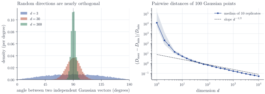
\[\cos\theta = \frac{\inner{Z}{Z'}}{\norm Z\norm{Z'}} = \frac{N}{\norm Z}, \qquad N \sim N(0,1),\]and \(\cos^2\theta\) is the squared length of the projection of the random unit vector \(Z/\norm Z\) on a fixed line, which has the \(\mathrm{Beta}(1/2, (d-1)/2)\) distribution with mean \(1/d\). Combining with Theorem 2, \(\sqrt d\cos\theta\) converges in distribution to \(N(0,1)\), so the angle is \(\pi/2 + O_P(d^{-1/2})\) (Figure 2, left). In the plane two random directions make any angle with equal probability; in dimension 300 the angle is within five degrees of a right angle with probability about 0.87.
A quantitative consequence: a set of \(m\) independent random unit vectors has all pairwise inner products bounded by \(t\) in absolute value with probability at least \(1 - m^2e^{-c\,dt^2}\) for an absolute constant \(c > 0\). So \(\R^d\) contains exponentially many nearly orthogonal directions, although it contains only \(d\) exactly orthogonal ones. This is the phenomenon behind random projections and the Johnson–Lindenstrauss lemma.
Distances lose their contrast
For independent \(Z, Z' \sim N(0, I_d)\), the difference \(Z - Z'\) is \(N(0, 2I_d)\), so Theorem 2 applies to \(\norm{Z - Z'}^2/2\). Take \(n\) independent points and apply the union bound to the \(\binom n2\) pairs:
\[\P\Bigl(\text{some pair has } \Bigl\lvert\frac{\norm{Z_i - Z_j}^2}{2d} - 1\Bigr\rvert \ge t\Bigr) \le n^2e^{-dt^2/8}.\]Choosing \(t = \sqrt{8(2\log n + \log(1/\delta))/d}\), which is at most one when \(d\) is large compared with \(\log(n/\delta)\), shows that with probability at least \(1 - \delta\) all squared distances lie in \(2d(1 \pm t)\). The ratio between the largest and the smallest pairwise distance is then at most \(\sqrt{(1+t)/(1-t)} = 1 + O\bigl(\sqrt{\log(n/\delta)/d}\bigr)\). The right panel of Figure 2 shows the relative contrast \((D_{\max} - D_{\min})/D_{\min}\) among 100 Gaussian points decaying at rate \(d^{-1/2}\).
When every point is at nearly the same distance from every other, the nearest neighbour of a query point is barely nearer than the farthest, and methods built on distances (nearest-neighbour classification, kernel smoothing with isotropic kernels, clustering) carry little information unless the data have low-dimensional structure. The calculation assumes isotropic noise in all \(d\) coordinates; real data that concentrate near a low-dimensional set behave like data in that lower dimension, which is why such methods often still work.
Remarks
All of these facts are instances of the concentration of measure phenomenon: Lipschitz functions of many independent variables are nearly constant. The Gaussian Poincaré inequality gives \(\Var f(Z) \le \E\norm{\nabla f(Z)}^2\), hence \(\Var\norm Z \le 1\), and the Gaussian concentration inequality gives \(\P(\abs{f(Z) - \E f(Z)} \ge s) \le 2e^{-s^2/2}\) for every 1-Lipschitz \(f\); applied to \(f(z) = \norm z\) with \(s = t\sqrt d\) it improves the exponent in the second bound of Theorem 2 from \(dt^2/8\) to \(dt^2/2\), for deviations measured from \(\E\norm Z \in [\sqrt{d-1}, \sqrt d]\) and for all \(t > 0\). R. Vershynin, High-Dimensional Probability, develops this theory with statistical applications, and A. Blum, J. Hopcroft and R. Kannan, Foundations of Data Science, has an accessible chapter on high-dimensional geometry. A precise version of the chi-squared tail bound with explicit constants is due to B. Laurent and P. Massart, “Adaptive estimation of a quadratic functional by model selection” (Annals of Statistics, 2000).