Hamiltonian Monte Carlo: momentum, the leapfrog map and an exact accept–reject step

Random-walk Metropolis proposes $q' = q + h\xi$ with $\xi$ standard normal. The scale $h$ must be of the order of the narrowest direction of the target, or almost every proposal is rejected, and a random walk with steps of size $h$ needs about $(\ell/h)^2$ iterations to cover a distance $\ell$. Long, thin or high-dimensional posteriors therefore mix slowly. Hamiltonian Monte Carlo (HMC) uses the gradient of the log density to build proposals that travel a long way along the target and are still accepted with high probability. The method leaves the target exactly invariant for any choice of its two tuning parameters, the step size and the number of steps, and a Gaussian target, for which everything can be computed in closed form, shows how both parameters govern efficiency.

The augmented target

Let the target on $\R^d$ be $\pi(q) \propto \exp\{-U(q)\}$, where the potential $U$ is twice continuously differentiable and bounded below. Introduce an auxiliary momentum $p \in \R^d$, independent of $q$, with $p \sim N(0, M)$ for a symmetric positive definite mass matrix $M$. The joint density is

\[\rho(q, p) \propto \exp\{-H(q, p)\}, \qquad H(q, p) = U(q) + \tfrac12 p^\top M^{-1} p,\]

and its $q$-marginal is $\pi$. Any Markov chain that leaves $\rho$ invariant yields a chain for $\pi$ by discarding the momenta.

Hamiltonian dynamics

The Hamiltonian flow $\varphi_t$ is the solution map of

\[\frac{\dd q}{\dd t} = M^{-1} p, \qquad \frac{\dd p}{\dd t} = -\nabla U(q).\]

Since $\nabla U$ is $C^1$, solutions exist and are unique locally. The flow has three properties.

Energy conservation. Along a solution, $\frac{\dd}{\dd t} H = \nabla U(q)^\top M^{-1} p + p^\top M^{-1}\bigl(-\nabla U(q)\bigr) = 0$. Because $U$ is bounded below, the kinetic energy and hence $p$ stay bounded, so $q$ grows at most linearly and solutions exist for all $t$.
Volume preservation. The vector field $(M^{-1}p, -\nabla U(q))$ has divergence $\nabla_q \cdot M^{-1}p - \nabla_p \cdot \nabla U(q) = 0$, so by Liouville’s theorem $\det D\varphi_t = 1$.
Reversibility. With $F(q, p) = (q, -p)$, if $(q(t), p(t))$ solves the equations then so does $(q(-t), -p(-t))$. Hence $F \circ \varphi_t \circ F = \varphi_{-t}$, and $F \circ \varphi_t$ is its own inverse.

Moving along the exact flow keeps $\rho$ unchanged, and the momentum, redrawn at each iteration, changes the energy level so that the chain is not confined to one level set of $H$. The exact flow is rarely available, so it is replaced by a numerical integrator that keeps properties 2 and 3 exactly and property 1 only approximately.

The leapfrog map

One leapfrog step of size $\varepsilon$ is the composition $\Phi_\varepsilon = K \circ D \circ K$ of a half kick, a full drift and a half kick:

\[K(q, p) = \bigl(q,\; p - \tfrac{\varepsilon}{2} \nabla U(q)\bigr), \qquad D(q, p) = \bigl(q + \varepsilon M^{-1} p,\; p\bigr).\]

Each factor is a shear. The Jacobian matrix of $K$ is block lower triangular with identity blocks on the diagonal, and that of $D$ is block upper triangular with identity diagonal blocks, so both have determinant one, and so has $\Phi_\varepsilon$. For reversibility, a direct computation gives $F K F (q, p) = (q, p + \tfrac\varepsilon2 \nabla U(q)) = K^{-1}(q, p)$ and $F D F(q, p) = (q - \varepsilon M^{-1}p, p) = D^{-1}(q, p)$. Since $F^2$ is the identity,

\[F \Phi_\varepsilon F = (FKF)(FDF)(FKF) = K^{-1} D^{-1} K^{-1} = \Phi_\varepsilon^{-1}.\]

Iterating, $F \Phi_\varepsilon^L F = \Phi_\varepsilon^{-L}$, so the proposal map $\Psi = F \circ \Phi_\varepsilon^L$ satisfies $\Psi \circ \Psi = \mathrm{id}$. It is a $C^1$ involution with Jacobian determinant of absolute value one. Energy is not conserved: for smooth $U$ the leapfrog energy error over a fixed integration time $L\varepsilon$ is of order $\varepsilon^2$ on bounded sets (Hairer, Lubich and Wanner, Geometric Numerical Integration). The Metropolis step removes this error exactly.

Exactness

Lemma 1. Let $\rho$ be a positive probability density on $\R^{m}$ and $\Psi : \R^m \to \R^m$ a $C^1$ map with $\Psi \circ \Psi = \mathrm{id}$ and $\abs{\det D\Psi} \equiv 1$. The kernel that moves from $z$ to $\Psi(z)$ with probability $a(z) = \min\{1, \rho(\Psi(z))/\rho(z)\}$ and otherwise stays at $z$ is reversible with respect to $\rho$.

Proof. Let $Z \sim \rho$ and let $Z'$ be the next state. For bounded measurable $f, g$,

\[\E\bigl[f(Z) g(Z')\bigr] = \int f(z)\, g(\Psi(z))\, \min\{\rho(z), \rho(\Psi(z))\}\, \dd z + \int f(z) g(z) \bigl(1 - a(z)\bigr)\rho(z)\, \dd z .\]

The second term is symmetric in $f$ and $g$. In the first, $\Psi$ is a $C^1$ bijection (it is its own inverse) with unit absolute Jacobian, so the substitution $z = \Psi(w)$ gives $\dd z = \dd w$ and, using $\Psi(\Psi(w)) = w$,

\[\int f(\Psi(w))\, g(w)\, \min\{\rho(\Psi(w)), \rho(w)\}\, \dd w ,\]

which is the first term with $f$ and $g$ exchanged. Hence $\E[f(Z) g(Z')] = \E[g(Z) f(Z')]$.

An HMC iteration from state $q$ consists of three steps: draw $p \sim N(0, M)$, which is a Gibbs update of the momentum and leaves $\rho$ invariant; apply the kernel of Lemma 1 with $\Psi = F \circ \Phi_\varepsilon^L$; discard $p$. Because $H(F z) = H(z)$, the acceptance probability is $\min\{1, \exp(H(z) - H(\Phi_\varepsilon^L z))\}$, and the flip $F$ never needs to be applied since the next momentum is drawn afresh. With $M = I$:

def hmc_step(q, logp, grad_logp, eps, L, rng):
    p = rng.standard_normal(q.shape)
    q_new, p_new = q.copy(), p.copy()
    p_new += 0.5 * eps * grad_logp(q_new)
    for k in range(L):
        q_new += eps * p_new
        if k < L - 1:
            p_new += eps * grad_logp(q_new)  # two half kicks merged
    p_new += 0.5 * eps * grad_logp(q_new)
    log_ratio = logp(q_new) - 0.5 * p_new @ p_new - logp(q) + 0.5 * p @ p
    return q_new if np.log(rng.random()) < log_ratio else q

Lemma 1 holds whatever the values of $\varepsilon$ and $L$. They affect only efficiency, and the Gaussian case shows exactly how.

Step size: the Gaussian case solved

Take $d = 1$, $M = 1$ and $U(q) = q^2/(2\sigma^2)$. The leapfrog step is linear, $\Phi_\varepsilon(q, p) = A(q, p)^\top$, and composing the three shears gives

\[A = \begin{pmatrix} a & \varepsilon \\ -\dfrac{\varepsilon c}{\sigma^2} & a \end{pmatrix}, \qquad a = 1 - \frac{\varepsilon^2}{2\sigma^2}, \qquad c = 1 - \frac{\varepsilon^2}{4\sigma^2}.\]

Proposition 2. Let $(q_k, p_k) = \Phi_\varepsilon^k(q_0, p_0)$.

If $\varepsilon < 2\sigma$, the quadratic form $\tilde H(q, p) = \tfrac12 p^2 + c\, q^2/(2\sigma^2)$ is conserved exactly, and $H(q_k, p_k) - H(q_0, p_0) = \varepsilon^2 (q_k^2 - q_0^2)/(8\sigma^4)$. The energy error is $O(\varepsilon^2)$ uniformly in $k$.
If $\varepsilon > 2\sigma$, $A$ has a real eigenvalue $\lambda$ with $\abs{\lambda} > 1$, and $\norm{(q_k, p_k)}$ grows like $\abs\lambda^k$ for every initial point off the eigenline of the other eigenvalue.

Proof. Write $q' = a q + \varepsilon p$ and $p' = a p - \varepsilon c q/\sigma^2$. In $c q'^2/\sigma^2 + p'^2$ the cross terms $2 a \varepsilon c\, q p/\sigma^2$ cancel, the coefficient of $p^2$ is $a^2 + \varepsilon^2 c/\sigma^2$ and that of $q^2$ is $(c/\sigma^2)(a^2 + \varepsilon^2 c/\sigma^2)$. Expanding,

\[a^2 + \frac{\varepsilon^2 c}{\sigma^2} = 1 - \frac{\varepsilon^2}{\sigma^2} + \frac{\varepsilon^4}{4\sigma^4} + \frac{\varepsilon^2}{\sigma^2} - \frac{\varepsilon^4}{4\sigma^4} = 1,\]

so $\tilde H$ is invariant under $A$ for every $\varepsilon$. When $\varepsilon < 2\sigma$ we have $c > 0$, and $H - \tilde H = (1 - c) q^2/(2\sigma^2) = \varepsilon^2 q^2/(8\sigma^4)$ gives the identity in part 1. The level sets of $\tilde H$ are then ellipses, so $q_k^2 \le 2\sigma^2 \tilde H(q_0, p_0)/c$ for all $k$, which gives the uniform bound.

For part 2, $\det A = a^2 + \varepsilon^2 c/\sigma^2 = 1$ by the display above, and $\tr A = 2a = 2 - \varepsilon^2/\sigma^2$. The eigenvalues solve $\lambda^2 - (\tr A)\lambda + 1 = 0$. If $\varepsilon > 2\sigma$ then $\tr A < -2$, the roots are real with product one, and one of them has modulus greater than one. Decomposing $(q_0, p_0)$ in the eigenbasis gives the growth statement.

For $U(q) = \tfrac12 q^\top \Sigma^{-1} q$ in $\R^d$ with $M = I$, an orthogonal change of coordinates diagonalizes $\Sigma$ and commutes with each leapfrog substep, so the dynamics split into $d$ independent one-dimensional problems with standard deviations $\sigma_1, \dots, \sigma_d$. The integrator is stable only if $\varepsilon < 2\sigma_{\min}$, while covering the widest direction takes an integration time of order $\sigma_{\max}$. The number of gradient evaluations per iteration is therefore at least of order $\sigma_{\max}/\sigma_{\min}$, the square root of the condition number of $\Sigma$. Choosing $M^{-1}$ close to the posterior covariance removes this factor, which is why practical implementations adapt the mass matrix during warm-up.

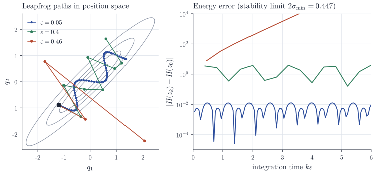
Leapfrog paths for three step sizes on a correlated Gaussian, and the corresponding energy errors on a log scale — Figure 1. Target $N(0, \Sigma)$ with unit variances and correlation $0.95$, so $\sigma_{\min} = \sqrt{0.05}$. Left: leapfrog paths in position space from the same $(q_0, p_0)$, with 64, 8 and 3 steps. Right: absolute energy error along longer paths. For $\varepsilon = 0.05$ the error stays near $10^{-2}$; for $\varepsilon = 0.4$, just below the limit $0.447$, the path remains bounded but the energy error is of order one; for $\varepsilon = 0.46$ it grows geometrically.

Figure 1 shows both regimes. The error does not accumulate with the number of steps when the integrator is stable, as part 1 of Proposition 2 predicts, but its size depends on how close $\varepsilon$ is to the limit through the factor $1/c$. In high dimension the energy error is a sum over many coordinates, and Beskos, Pillai, Roberts, Sanz-Serna and Stuart (Bernoulli, 2013) show for product targets that $\varepsilon$ should scale as $d^{-1/4}$, with an optimal acceptance probability of about $0.651$.

Integration time

The second tuning parameter is $T = L\varepsilon$. For the one-dimensional Gaussian the exact flow is a rotation,

\[q(T) = q_0 \cos(T/\sigma) + \sigma p_0 \sin(T/\sigma).\]

Start in stationarity, $q_0 = \sigma X$ and $p_0 = Y$ with $X, Y$ independent standard normal, and write $C = \cos(T/\sigma)$, $S = \sin(T/\sigma)$. Then $q(T)/\sigma = CX + SY$ is again standard normal, and

\[\begin{aligned} \Corr\bigl(q_0, q(T)\bigr) &= \Cov(X, CX + SY) = C, \\ \Corr\bigl(q_0^2, q(T)^2\bigr) &= \frac{\Cov(X^2,\, C^2X^2 + 2CS\,XY + S^2Y^2)}{\Var(X^2)} = \frac{2C^2}{2} = C^2, \end{aligned}\]

using $\Cov(X^2, XY) = \E X^3 \E Y = 0$ and $\Cov(X^2, Y^2) = 0$. These are the lag-one autocorrelations of HMC with exact dynamics. At $T = \pi\sigma/2$ consecutive states are independent. At $T = \pi\sigma$ the chain is perfectly antithetic for $q$, which makes the ergodic average of $q$ very accurate, while $q^2$ does not change at all. At $T = 2\pi\sigma$ the chain returns to its starting point and does not move. With leapfrog dynamics and a small step the picture is the same, as the simulated points in Figure 2 confirm.

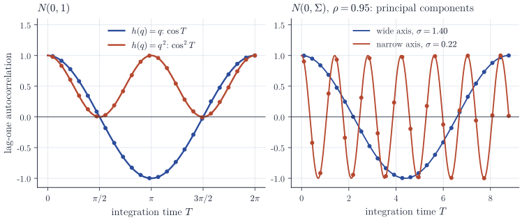
Lag-one autocorrelation of HMC as a function of integration time for a one-dimensional Gaussian and for the two principal axes of a correlated Gaussian — Figure 2. Lag-one autocorrelation of HMC as a function of the integration time $T$. Curves are the exact-flow values; points are estimates from $20{,}000$ independent HMC transitions started in stationarity, using leapfrog with $\varepsilon = 0.05$ (left) and $\varepsilon = 0.1\,\sigma_{\min}$ (right). Left: $N(0,1)$, for $q$ and $q^2$. Right: the target of Figure 1 along its principal axes, where the narrow coordinate oscillates about six times faster than the wide one.

In several dimensions the coordinates rotate at frequencies $1/\sigma_i$, and no single $T$ is good for all of them (right panel). With exact dynamics, a fixed $T$ equal to $\pi\sigma_i$ merely negates the $i$th principal coordinate at every iteration, so its square never changes and the chain is not ergodic; leapfrog dynamics behave in nearly the same way. Drawing $L$ or $\varepsilon$ at random at each iteration avoids exact periodicities, and the no-U-turn sampler of Hoffman and Gelman (Journal of Machine Learning Research, 2014) chooses the path length adaptively, stopping the trajectory when it starts to turn back on itself.

Remarks

Hamiltonian Monte Carlo originated in lattice field theory as hybrid Monte Carlo (Duane, Kennedy, Pendleton and Roweth, Physics Letters B, 1987). Neal’s chapter “MCMC using Hamiltonian dynamics” in the Handbook of Markov Chain Monte Carlo (2011) is the standard statistical introduction, and Betancourt’s “A conceptual introduction to Hamiltonian Monte Carlo” (2017) develops the geometric point of view. The exactness argument uses only that the proposal map is a volume-preserving involution, so it applies unchanged to any reversible, volume-preserving integrator composed with the momentum flip.