Perturb and maximize: sampling a categorical distribution with Gumbel noise

October 12, 2026Probability

Suppose we want a draw from the categorical distribution on \(\{1, \dots, K\}\) with probabilities

\[\pi_k = \frac{e^{a_k}}{\sum_{j=1}^K e^{a_j}}, \qquad a_1, \dots, a_K \in \R .\]

The numbers \(a_k\) are typically available only up to an additive constant: log-likelihoods plus log-prior weights, logits of a classifier, negative energies. The usual method normalizes, forms the cumulative sums and inverts at a uniform draw. The Gumbel-max trick does something that looks different: it adds independent noise to each \(a_k\) and reports the index of the largest perturbed value. No normalization and no cumulative sum are needed, and the computation stays in log space. The draw is exact, and one short calculation proves this and also yields sampling without replacement and a differentiable relaxation.

The Gumbel distribution

A real random variable \(G\) has the standard Gumbel distribution if

\[\P(G \le x) = \exp\bigl(-e^{-x}\bigr), \qquad x \in \R,\]

with density \(e^{-x}\exp(-e^{-x})\). It is the limit law of suitably centred maxima of many light-tailed variables, for example \(\max_{i \le n} E_i - \log n\) for independent standard exponentials \(E_i\). If \(U\) is uniform on \((0, 1)\) then \(-\log(-\log U)\) is standard Gumbel, since \(\P(-\log(-\log U) \le x) = \P(U \le \exp(-e^{-x}))\). We write \(\mathrm{Gumbel}(m)\) for the law of \(m + G\).

The main result

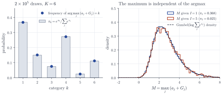
Theorem 1. Let \(G_1, \dots, G_K\) be independent standard Gumbel variables, \(Y_k = a_k + G_k\), \(I = \arg\max_k Y_k\) and \(M = \max_k Y_k\), and let \(S = \sum_j e^{a_j}\). Then \(I\) is almost surely well defined and

1. \(\P(I = k) = \pi_k\) for each \(k\);
2. \(M \sim \mathrm{Gumbel}(\log S)\);
3. \(I\) and \(M\) are independent.

Proof. The \(Y_k\) are independent with continuous distributions, so ties occur with probability zero. Each \(Y_j\) has distribution function \(F_j(y) = \exp(-e^{-(y - a_j)})\), and therefore

\[\prod_{j=1}^K F_j(y) = \exp\Bigl(-e^{-y} \sum_{j} e^{a_j}\Bigr) = \exp\bigl(-S e^{-y}\bigr).\]

The event \(\{I = k, M \le m\}\) is the event that \(Y_k \le m\) and \(Y_j < Y_k\) for all \(j \ne k\). Conditioning on \(Y_k = y\) and using independence,

\[\P(I = k,\, M \le m) = \int_{-\infty}^{m} e^{-(y - a_k)} \exp\bigl(-e^{-(y - a_k)}\bigr) \prod_{j \ne k} F_j(y)\, \dd y = \int_{-\infty}^{m} e^{a_k} e^{-y} \exp\bigl(-S e^{-y}\bigr)\, \dd y .\]

The integrand is \((e^{a_k}/S)\) times the derivative of \(\exp(-S e^{-y})\), which tends to zero as \(y \to -\infty\). Hence

\[\P(I = k,\, M \le m) = \frac{e^{a_k}}{S}\, \exp\bigl(-e^{-(m - \log S)}\bigr) = \pi_k \cdot \P\bigl(\mathrm{Gumbel}(\log S) \le m\bigr).\]

Letting \(m \to \infty\) gives part 1, summing over \(k\) gives part 2, and the product form is part 3.

The only property of the Gumbel distribution used in the proof is that the product of the distribution functions of the shifted variables is again a shifted Gumbel distribution function, with shift \(\log \sum_j e^{a_j}\). This max-stability is what turns a sum of exponentials, the normalizing constant, into a maximum.

Part 2 also gives \(\E M = \log S + \gamma\), where \(\gamma\) is the Euler–Mascheroni constant, the mean of the standard Gumbel distribution. Hence \(M - \gamma\) is an unbiased estimator of the log-normalizer \(\log S\), which is the starting point of perturbation methods for estimating partition functions.

Figure 1. Gumbel-max sampling with $K = 6$ and $a = (1.2, 0.3, -0.4, 0.9, -1.5, 0)$. Left: target probabilities and frequencies of the argmax in $2 \times 10^5$ draws. Right: histograms of the maximum $M$ among draws whose argmax is category 1 and among draws whose argmax is category 5, a common event and a rare one, together with the $\mathrm{Gumbel}(\log S)$ density. The two conditional distributions coincide, as part 3 of Theorem 1 asserts.

Exponential clocks

The theorem has an equivalent form in terms of exponential random variables. If \(G\) is standard Gumbel then \(E = e^{-G}\) is standard exponential, because \(\P(e^{-G} > t) = \P(G < -\log t) = e^{-t}\) for \(t > 0\). Writing \(\lambda_k = e^{a_k}\),

\[Y_k = a_k + G_k = -\log\bigl(E_k / \lambda_k\bigr),\]

and \(T_k = E_k/\lambda_k\) is exponential with rate \(\lambda_k\). Since \(-\log\) is decreasing, the largest \(Y_k\) corresponds to the smallest \(T_k\). Theorem 1 thus says that among independent exponential clocks with rates \(\lambda_1, \dots, \lambda_K\), clock \(k\) rings first with probability \(\lambda_k / \sum_j \lambda_j\), the first ringing time is exponential with rate \(\sum_j \lambda_j\), and the identity of the first clock is independent of the time at which it rings. These are the familiar facts behind the construction of continuous-time Markov chains, and the Gumbel-max trick is their image under \(t \mapsto -\log t\).

Sampling without replacement

The clock picture also explains what the second largest perturbed value means.

Proposition 2. Let \(I_1, I_2, \dots, I_K\) be the indices of \(Y_1, \dots, Y_K\) in decreasing order. For distinct \(k_1, \dots, k_m\),

\[\P(I_1 = k_1, \dots, I_m = k_m) = \prod_{r=1}^{m} \frac{\lambda_{k_r}}{\sum_{j \notin \{k_1, \dots, k_{r-1}\}} \lambda_j } .\]

In particular, the indices of the \(m\) largest perturbed values form a sample of size \(m\) drawn sequentially without replacement with probabilities proportional to \(\lambda_k\).

Proof. Work with the clocks \(T_j = E_j/\lambda_j\), so that \(I_r\) is the index of the \(r\)-th clock to ring. Let \(\Lambda = \sum_j \lambda_j\). For \(t, s_j \ge 0\), independence gives

\[\P\bigl(T_k \in \dd t,\; T_j > t + s_j \text{ for } j \ne k\bigr) = \lambda_k e^{-\lambda_k t}\, \dd t \prod_{j \ne k} e^{-\lambda_j (t + s_j)} = \lambda_k e^{-\Lambda t}\, \dd t \prod_{j \ne k} e^{-\lambda_j s_j}.\]

The right-hand side factorizes: conditionally on the first clock being \(k\) and ringing at time \(t\), the residual times \(T_j - t\), \(j \ne k\), are independent exponentials with rates \(\lambda_j\). The remaining race therefore has the same structure with clock \(k\) removed, and by Theorem 1 the next clock to ring is \(j\) with probability \(\lambda_j/(\Lambda - \lambda_k)\). Induction on \(m\) gives the formula.

The ordering in Proposition 2 is the Plackett–Luce model for rankings. Kool, van Hoof and Welling (2019, International Conference on Machine Learning) use this observation, which they call the Gumbel-top-\(k\) trick, to draw samples without replacement from sequence models by a beam search over perturbed scores.

A differentiable relaxation

The map from \((a, G)\) to the one-hot vector \(e_I\) is piecewise constant in \(a\), so it carries no gradient information. Replacing the argmax by a softmax with temperature \(\tau > 0\),

\[x_\tau = \operatorname{softmax}\Bigl(\frac{a + G}{\tau}\Bigr), \qquad (x_\tau)_k = \frac{\exp\{(a_k + G_k)/\tau\}}{\sum_j \exp\{(a_j + G_j)/\tau\}},\]

gives a random point in the interior of the probability simplex that is a smooth function of \(a\) for each fixed \(G\). As \(\tau \to 0\), \(x_\tau \to e_I\) almost surely: the gap \(\Delta = Y_I - \max_{j \ne I} Y_j\) is positive almost surely, and \(1 - (x_\tau)_I \le (K - 1) e^{-\Delta/\tau}\). As \(\tau \to \infty\), \(x_\tau\) tends to the barycentre \((1/K, \dots, 1/K)\).

Figure 2. Fifteen hundred draws of $x_\tau$ for $\pi = (0.5, 0.3, 0.2)$, plotted in the probability simplex with vertices $e_1, e_2, e_3$ and coloured by the argmax $I$. At $\tau = 0.1$ the draws sit near the vertices with frequencies close to $\pi$; at $\tau = 5$ they collapse toward the centre, and the colour regions are the sectors where one coordinate is largest.

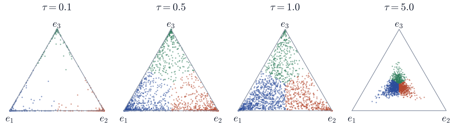
The law of \(x_\tau\) was introduced simultaneously as the Gumbel-softmax distribution by Jang, Gu and Poole and as the Concrete distribution by Maddison, Mnih and Teh (both ICLR 2017), with an explicit density on the simplex. It allows gradients of \(\E \ell(x_\tau)\) with respect to \(a\) to be estimated by differentiating through the sample. For \(\tau > 0\) these differ from gradients of \(\E \ell(e_I)\), the quantity of interest for a discrete latent variable, so the temperature trades bias (large \(\tau\)) against variance of the gradient estimates (small \(\tau\)). The score-function estimator, which is unbiased for the discrete objective, is the usual alternative.

Remarks

For a single draw from a fixed distribution, inverse-CDF sampling needs one uniform variable and Gumbel-max needs \(K\), so the trick is not about saving random numbers. Its advantages are that it works directly with unnormalized log-weights, avoiding overflow when the \(a_k\) are large; that the \(K\) perturbations can be generated and compared in parallel; and that the maximum, the argmax and the ordering carry the extra information described above. For many draws from the same distribution, the alias method is faster than either. Background on the Gumbel law as an extreme-value limit is in de Haan and Ferreira, Extreme Value Theory: An Introduction.