Updating beliefs with a loss instead of a likelihood: Gibbs posteriors and the learning rate
Bayesian inference about a parameter normally requires a model for the whole distribution of the data. Often the quantity of interest is defined more directly, as the minimizer of an expected loss. The population median minimizes \(\theta \mapsto \E\abs{X - \theta}\), a quantile minimizes the check loss, and a classifier’s parameter minimizes expected hinge loss. Writing a likelihood for such a problem forces assumptions about aspects of the distribution that are irrelevant to the target, and if those assumptions are wrong the posterior concentrates on the wrong quantity. Gibbs posteriors, also called generalized posteriors or quasi-posteriors, update a prior directly through the loss that defines the target.
Definition
Let \(X_1, \dots, X_n\) be independent with common distribution \(P\) on a space \(\mathcal X\), let \(\ell : \Theta \times \mathcal X \to \R\) be a loss that is measurable in both arguments, and define the target
\[\theta^\ast = \argmin_{\theta \in \Theta} R(\theta), \qquad R(\theta) = \E_P\, \ell(\theta, X),\]assumed to exist and be unique. With empirical loss \(L_n(\theta) = \sum_{i=1}^n \ell(\theta, X_i)\), a prior \(\pi\) on \(\Theta\) and a learning rate \(\omega > 0\), the Gibbs posterior is
\[\pi_n^\omega(\dd\theta) = \frac{e^{-\omega L_n(\theta)} \, \pi(\dd\theta)}{Z_n(\omega)}, \qquad Z_n(\omega) = \int_\Theta e^{-\omega L_n(\theta)} \, \pi(\dd\theta),\]defined whenever \(0 < Z_n(\omega) < \infty\). If \(\ell(\theta, x) = -\log p_\theta(x)\) for a statistical model \(\{p_\theta\}\) and \(\omega = 1\), this is the ordinary posterior; with \(\omega \ne 1\) it is a tempered or power posterior. The name comes from statistical mechanics, where a density proportional to \(e^{-\text{energy}/\text{temperature}}\) is a Gibbs measure, and \(1/\omega\) plays the role of temperature.
Two questions arise at once: why this form rather than some other function of the loss, and what value of \(\omega\) to use. The likelihood case gives no guidance on the second, because there \(\omega = 1\) is fixed by the model. With a general loss, \(\omega\) converts units of loss into units of log-probability, and nothing in the loss fixes the exchange rate.
A variational characterization
The answer to the first question is that \(\pi_n^\omega\) is the unique minimizer of an objective that trades fit to the data against distance from the prior.
Proposition 1. Suppose \(0 < Z_n(\omega) < \infty\), and let \(\mathcal Q\) be the set of probability measures \(\rho\) on \(\Theta\) with \(\KL(\rho \,\Vert\, \pi) < \infty\) and \(\int \abs{L_n} \, \dd\rho < \infty\). For \(\rho \in \mathcal Q\),
\[\omega \int L_n \, \dd\rho + \KL(\rho \,\Vert\, \pi) = \KL(\rho \,\Vert\, \pi_n^\omega) - \log Z_n(\omega).\]Consequently, if \(\pi_n^\omega \in \mathcal Q\), it is the unique minimizer over \(\mathcal Q\) of \(\rho \mapsto \omega \int L_n \, \dd\rho + \KL(\rho \,\Vert\, \pi)\), and the minimum value is \(-\log Z_n(\omega)\).
Proof. Let \(\rho \in \mathcal Q\), so that \(\rho \ll \pi\). Since \(\pi_n^\omega\) and \(\pi\) are mutually absolutely continuous with \(\dd\pi_n^\omega / \dd\pi = e^{-\omega L_n}/Z_n(\omega) > 0\), also \(\rho \ll \pi_n^\omega\) and
\[\log\frac{\dd\rho}{\dd\pi_n^\omega} = \log\frac{\dd\rho}{\dd\pi} + \omega L_n + \log Z_n(\omega) \qquad \rho\text{-almost everywhere}.\]The last two terms are \(\rho\)-integrable because \(\int\abs{L_n}\,\dd\rho < \infty\), and the first has \(\rho\)-integral \(\KL(\rho \,\Vert\, \pi) < \infty\); integrating against \(\rho\) therefore gives the identity, with all terms finite. The right-hand side is minimized exactly when \(\KL(\rho \,\Vert\, \pi_n^\omega) = 0\), that is, when \(\rho = \pi_n^\omega\).
Read this way, the Gibbs posterior is the solution of an optimization problem and requires no model for the data: among all distributions over \(\Theta\), it is the one with small expected empirical loss that is not too far from the prior in Kullback–Leibler divergence. The learning rate sets the relative weight of the two terms. The same objective appears in PAC-Bayesian bounds, where it controls the generalization error of randomized predictors (Catoni, PAC-Bayesian Supervised Classification). Bissiri, Holmes and Walker (2016, Journal of the Royal Statistical Society, Series B) argued from a different direction: if a rule for updating beliefs with a loss is to be coherent, in the sense that updating on two batches of data in turn gives the same result as updating on both at once, then, under their axioms, the update must have this exponential form, again leaving \(\omega\) free.
The learning rate controls the spread
To see what \(\omega\) does, consider the behaviour for large \(n\). Suppose \(R\) is twice differentiable at \(\theta^\ast\) with positive definite Hessian \(H\), and that \(\ell(\cdot, x)\) has a (sub)gradient \(g(\theta^\ast, x)\) at \(\theta^\ast\) with \(\E g(\theta^\ast, X) = 0\) and covariance \(J\). Let \(\hat\theta_n\) minimize \(L_n\), an M-estimator. Under regularity conditions, \(\sqrt n(\hat\theta_n - \theta^\ast)\) is asymptotically \(N(0, H^{-1}JH^{-1})\), the sandwich covariance. On the other hand, \(L_n(\theta) - L_n(\hat\theta_n) \approx \tfrac n2 (\theta - \hat\theta_n)^\top H (\theta - \hat\theta_n)\) for \(\theta\) within \(O(n^{-1/2})\) of \(\hat\theta_n\), so for fixed \(\omega\) and a prior with a density that is continuous and positive at \(\theta^\ast\), the Gibbs posterior is approximately
\[\pi_n^\omega \approx N\bigl(\hat\theta_n, \; (\omega n H)^{-1}\bigr),\]in the sense that the total variation distance between the two tends to zero in probability as \(n \to \infty\). Chernozhukov and Hong (2003, Journal of Econometrics) proved a Bernstein–von Mises theorem of this kind for quasi-posteriors, under conditions that allow non-smooth criteria such as the check loss of quantile regression. The posterior is centred at the right estimator, but its covariance \((\omega n H)^{-1}\) matches the sampling covariance \(H^{-1}JH^{-1}/n\) only if \(\omega H = HJ^{-1}H\), that is, only if \(J = H/\omega\). In one dimension this is achieved by
\[\omega^\ast = H/J .\]In several dimensions a scalar \(\omega\) can fix the overall scale but not the shape, unless \(J\) is proportional to \(H\). For a correctly specified likelihood, \(H\) and \(J\) are both the Fisher information, and \(\omega^\ast = 1\): the information identity is what makes \(\omega = 1\) correct for ordinary posteriors.
The median under absolute-error loss
Take \(\ell(\theta, x) = \abs{x - \theta}\) on \(\Theta = \R\), and suppose \(P\) has a distribution function \(F\) with a density \(f\) that is continuous and positive at the median \(m\). The risk is \(R(\theta) = \E\abs{X - \theta}\). Assume \(\E\abs{X} < \infty\), so that \(R\) is finite. For \(\theta < \theta'\) one has \(\abs{x - \theta'} - \abs{x - \theta} = \int_\theta^{\theta'} \bigl(\mathbf 1\{x < u\} - \mathbf 1\{x > u\}\bigr) \dd u\), and taking expectations (Fubini’s theorem applies because the integrand is bounded and the interval is finite) gives
\[R(\theta') - R(\theta) = \int_\theta^{\theta'} \bigl(P(X < u) - P(X > u)\bigr) \dd u = \int_\theta^{\theta'} \bigl(2F(u) - 1\bigr) \dd u ,\]where the second equality holds because \(P(X = u) > 0\) for at most countably many \(u\). Hence \(R'(\theta) = 2F(\theta) - 1\) at every continuity point of \(F\), in particular on a neighbourhood of \(m\), where \(P\) has a continuous density; \(R'\) vanishes at \(m\), and \(H = R''(m) = 2f(m)\). Since \(f(m) > 0\), the median is unique. The subgradient \(g(m, X) = \mathbf 1\{X < m\} - \mathbf 1\{X > m\}\) takes the values \(\pm 1\) with probability \(\tfrac12\) each, so \(J = 1\). The calibrated learning rate is therefore
\[\omega^\ast = 2f(m),\]and the sandwich variance \(J/(H^2 n) = 1/(4f(m)^2 n)\) is the familiar asymptotic variance of the sample median.
The same identity, applied to the empirical distribution, describes the Gibbs posterior exactly. The density of \(\pi_n^\omega\) relative to \(\pi\) is proportional to \(\exp\{-\omega \sum_i \abs{X_i - \theta}\}\), whose logarithm is concave and piecewise linear, with slope \(\omega\bigl(\#\{i : X_i > \theta\} - \#\{i : X_i < \theta\}\bigr)\) between data points. With a flat prior near the sample median \(\hat m_n\), the log-density relative to its value at \(\hat m_n\) is
\[\begin{aligned} -\omega \int_{\hat m_n}^{\theta} \bigl(\#\{i : X_i < u\} - \#\{i : X_i > u\}\bigr) \dd u &= -\omega n \int_{\hat m_n}^{\theta} \bigl(2F_n(u) - 1\bigr) \dd u \\ &\approx -\omega n f(m) (\theta - \hat m_n)^2, \end{aligned}\]where \(F_n\) is the empirical distribution function. For \(\theta - \hat m_n\) of order \(n^{-1/2}\), the increment \(F_n(u) - F_n(\hat m_n)\) equals \(f(m)(u - \hat m_n)\) up to an error of order \(n^{-3/4}\) in probability (the increment of the empirical process \(\sqrt n(F_n - F)\) over an interval of length \(n^{-1/2}\) is of order \(n^{-1/4}\)), and \(F_n(\hat m_n)\) is within \(1/n\) of \(\tfrac12\), which gives the approximation. The Gibbs posterior is thus close to \(N\bigl(\hat m_n, 1/(2\omega n f(m))\bigr)\), whose variance equals the sampling variance \(1/(4f(m)^2n)\) exactly when \(\omega = 2f(m)\). For other \(\omega\) the ratio of the posterior standard deviation to the sampling standard deviation is \(\sqrt{\omega^\ast/\omega}\), so an equal-tailed \(95\%\) credible interval has asymptotic coverage
\[2\,\Phi\bigl(1.96\sqrt{\omega^\ast/\omega}\bigr) - 1 .\]Figure 1 checks this with data from a \(\mathrm{Gamma}(2, 1)\) distribution, for which \(m \approx 1.678\), \(f(m) \approx 0.313\) and \(\omega^\ast \approx 0.627\). The prior is uniform on \([0, 8]\), and all computations are exact on a fine grid. The left panel contrasts the Gibbs posteriors with what a convenient Gaussian model would give: a normal likelihood with flat prior on its mean (and the variance set to the sample variance) produces a posterior centred near the sample mean, which estimates the population mean \(2\). That is a different parameter. No amount of data moves it to the median, because a Gaussian likelihood defines its target as the mean whatever the true distribution.
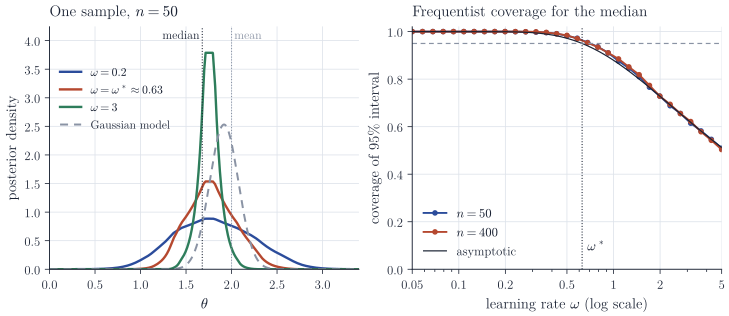
The right panel shows coverage over 2000 replications. The simulated curves for \(n = 50\) and \(n = 400\) lie almost on top of the asymptotic formula and cross \(0.95\) near \(\omega^\ast\). Choosing \(\omega = 1\), the value that looks natural by analogy with likelihoods, gives about 88% coverage here; \(\omega = 5\) gives about 50%.
Choosing the learning rate in practice
The calibrated value depends on the unknown \(f(m)\), and in general on the unknown \(H\) and \(J\). Several strategies are in use. A plug-in rule estimates \(H\) and \(J\) and sets \(\omega = \hat H/\hat J\) in one dimension. Syring and Martin (2019, Biometrika) choose \(\omega\) by bootstrap so that credible regions attain nominal frequentist coverage. Holmes and Walker (2017, Biometrika) match the expected information in the Gibbs posterior to that of a reference Bayesian update. Grünwald and van Ommen (2017, Bayesian Analysis) study power posteriors under misspecification and show that \(\omega < 1\) can be needed even with a likelihood-based loss; their SafeBayes method selects \(\omega\) from the data by a predictive criterion. These rules answer different questions, calibration of uncertainty versus quality of prediction, and need not agree.
Remarks
In this construction the target is defined by the loss, and the prior expresses beliefs about the target alone; no model is needed for the rest of the distribution of the data. The price is the calibration of uncertainty that a correctly specified likelihood provides automatically through the information identity, which the learning rate has to supply instead. Proposition 1 also shows that variational Bayes and Gibbs posteriors are the same optimization problem viewed from two sides: restricting \(\rho\) to a tractable family gives the usual variational approximation, now to a loss-based target.