Gaussian process regression as conditioning a Gaussian vector

October 12, 2026Machine learning

Nonparametric regression asks for an unknown function \(f\) from noisy evaluations \(y_i = f(x_i) + \varepsilon_i\). A Gaussian process prior makes the Bayesian version of this problem exactly solvable: the prior is specified through finite-dimensional Gaussian distributions, the data are linear functionals of \(f\) plus Gaussian noise, and all posterior computations reduce to one identity about conditioning jointly Gaussian vectors. That identity yields the posterior process in closed form, and the same Gaussian calculation gives the marginal likelihood used to choose the kernel.

Gaussian processes

Let \(\mathcal X\) be a set. A function \(k : \mathcal X \times \mathcal X \to \R\) is a positive semidefinite kernel if it is symmetric and \(\sum_{i,j} c_i c_j k(x_i, x_j) \ge 0\) for every finite collection \(x_1, \dots, x_n \in \mathcal X\) and \(c \in \R^n\). A real-valued stochastic process \((f(x))_{x \in \mathcal X}\) is a Gaussian process with mean function \(m\) and covariance function \(k\), written \(f \sim \mathcal{GP}(m, k)\), if for every finite \(x_1, \dots, x_n\)

\[\bigl(f(x_1), \dots, f(x_n)\bigr) \sim \mathcal N_n\bigl(m(\mathbf x), K(\mathbf x, \mathbf x)\bigr), \qquad K(\mathbf x, \mathbf x)_{ij} = k(x_i, x_j).\]

Such a process exists for every function \(m\) and every positive semidefinite \(k\). The prescribed finite-dimensional distributions are consistent: permuting the points permutes the coordinates of the Gaussian vector, and dropping a point marginalizes a Gaussian vector, which deletes the corresponding entry of the mean and row and column of the covariance. Kolmogorov’s extension theorem then gives a probability measure on \(\R^{\mathcal X}\) with the product \(\sigma\)-field having these finite-dimensional distributions. Conversely, the covariance function of any process with finite second moments is positive semidefinite, since \(\sum_{i,j} c_ic_j k(x_i,x_j) = \Var\bigl(\sum_i c_i f(x_i)\bigr)\).

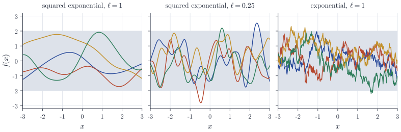
The finite-dimensional distributions do not determine path properties such as continuity, which concern uncountably many coordinates. For \(\mathcal X = \R\) these are settled by the Kolmogorov–Chentsov criterion applied to the increments. Two kernels illustrate the range. The squared exponential kernel

\[k(x, x') = \sigma_f^2 \exp\Bigl( -\frac{(x - x')^2}{2\ell^2} \Bigr)\]

gives \(\E\bigl(f(x) - f(x')\bigr)^2 = 2\sigma_f^2\bigl(1 - e^{-h^2/(2\ell^2)}\bigr) \le \sigma_f^2 h^2/\ell^2\) with \(h = \abs{x - x'}\). Together with the Gaussian moment identity \(\E\abs{Z}^{2m} = c_m (\Var Z)^m\) this gives a continuous version, and a finer analysis shows that there is a version with infinitely differentiable paths. The exponential kernel \(k(x,x') = \sigma_f^2 e^{-\abs{x-x'}/\ell}\) gives an increment variance of order \(h\), which by the same moment identity yields continuous versions whose paths are Hölder of every order below \(1/2\); on \(\R\) this is the stationary Ornstein–Uhlenbeck process, whose paths are almost surely nowhere differentiable. The length-scale \(\ell\) sets the distance over which values are strongly correlated.

Figure 1. Draws from zero-mean Gaussian process priors with $\sigma_f = 1$; the shaded band is $\pm 2\sigma_f$. A shorter length-scale gives faster variation; the exponential kernel gives rough paths.

Conditioning a Gaussian vector

Everything below rests on one lemma.

Lemma 1. Let \((U, V)\) be jointly Gaussian in \(\R^{p} \times \R^{q}\) with means \(\mu_U, \mu_V\) and covariance blocks \(\Sigma_{UU}, \Sigma_{UV}, \Sigma_{VV}\), and suppose \(\Sigma_{VV}\) is invertible. Then

\[U \mid V = v \;\sim\; \mathcal N\bigl( \mu_U + \Sigma_{UV}\Sigma_{VV}^{-1}(v - \mu_V),\; \Sigma_{UU} - \Sigma_{UV}\Sigma_{VV}^{-1}\Sigma_{VU} \bigr).\]

Proof. Let \(A = \Sigma_{UV}\Sigma_{VV}^{-1}\) and \(W = U - AV\). Then \(\Cov(W, V) = \Sigma_{UV} - A\Sigma_{VV} = 0\). The pair \((W, V)\) is a linear image of \((U, V)\) and hence jointly Gaussian, so zero covariance implies that \(W\) and \(V\) are independent. Thus, given \(V = v\), \(U = W + Av\) has the unconditional law of \(W\) shifted by \(Av\). That law is Gaussian with mean \(\mu_U - A\mu_V\) and covariance \(\Sigma_{UU} - A\Sigma_{VU} - \Sigma_{UV}A^\top + A\Sigma_{VV}A^\top = \Sigma_{UU} - \Sigma_{UV}\Sigma_{VV}^{-1}\Sigma_{VU}\).

The conditional covariance is the Schur complement of \(\Sigma_{VV}\), which is positive semidefinite and smaller than \(\Sigma_{UU}\) in the semidefinite order: conditioning never increases uncertainty, and the reduction does not depend on the observed value \(v\).

The posterior process

Take \(f \sim \mathcal{GP}(0, k)\) (a known mean function is subtracted from the data), inputs \(\mathbf x = (x_1, \dots, x_n)\) and

\[y_i = f(x_i) + \varepsilon_i, \qquad \varepsilon_1, \dots, \varepsilon_n \iid \mathcal N(0, \sigma^2), \quad \varepsilon \indep f,\]

with \(\sigma^2 > 0\). Write \(K = K(\mathbf x, \mathbf x)\), \(K_y = K + \sigma^2 I_n\) (positive definite), and \(k(x, \mathbf x) = \bigl(k(x, x_1), \dots, k(x, x_n)\bigr)\).

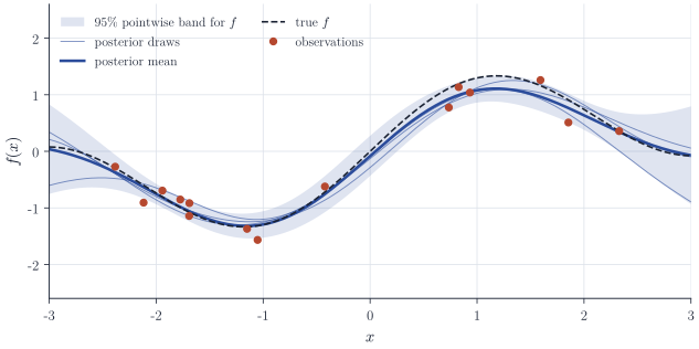
Proposition 2. Conditionally on \(y\), \(f\) is a Gaussian process with mean and covariance functions

\[\begin{aligned} m_{\mathrm{post}}(x) &= k(x, \mathbf x) K_y^{-1} y, \\ k_{\mathrm{post}}(x, x') &= k(x, x') - k(x, \mathbf x) K_y^{-1} k(\mathbf x, x'). \end{aligned}\]

Proof. Fix test points \(t_1, \dots, t_p\) and let \(U = (f(t_1), \dots, f(t_p))\), \(V = y\). Since \((U, f(x_1), \dots, f(x_n))\) is Gaussian and \(\varepsilon\) is an independent Gaussian vector, \((U, V)\) is jointly Gaussian with \(\Sigma_{VV} = K_y\), \(\Sigma_{UV} = K(\mathbf t, \mathbf x)\) and \(\Sigma_{UU} = K(\mathbf t, \mathbf t)\). Lemma 1 gives \(U \mid y \sim \mathcal N\bigl(K(\mathbf t, \mathbf x)K_y^{-1}y,\; K(\mathbf t,\mathbf t) - K(\mathbf t, \mathbf x)K_y^{-1}K(\mathbf x, \mathbf t)\bigr)\), which are the finite-dimensional distributions of \(\mathcal{GP}(m_{\mathrm{post}}, k_{\mathrm{post}})\). To make the statement precise, let \(Q_y\) denote the law of \(\mathcal{GP}(m_{\mathrm{post}}, k_{\mathrm{post}})\) on \(\R^{\mathcal X}\); it depends measurably on \(y\) because \(m_{\mathrm{post}}\) and \(k_{\mathrm{post}}\) do. For a cylinder set \(C = \{g : (g(t_1), \dots, g(t_p)) \in B\}\) and a Borel set \(D \subseteq \R^n\), the computation above gives \(\P(f \in C, y \in D) = \E[Q_y(C)\mathbf 1\{y \in D\}]\). Cylinder sets form a \(\pi\)-system generating the product \(\sigma\)-field, so by the \(\pi\)–\(\lambda\) theorem the identity extends to every measurable \(C\), and \(y \mapsto Q_y\) is a regular conditional distribution of \(f\) given \(y\).

Three features of these formulas matter in practice. First, with \(\alpha = K_y^{-1}y\) the posterior mean is \(m_{\mathrm{post}}(x) = \sum_{i=1}^n \alpha_i\, k(x, x_i)\), a combination of \(n\) kernel functions centred at the inputs, whatever the size of \(\mathcal X\). It coincides with the kernel ridge regression estimator that minimizes \(\sum_i (y_i - g(x_i))^2 + \sigma^2 \norm{g}_{\mathcal H}^2\) over the reproducing kernel Hilbert space of \(k\), which is how the noise variance acts as a regularization parameter. Second, \(k_{\mathrm{post}}\) depends on the inputs but not on the responses, so the width of the posterior bands is fixed before \(y\) is seen; under a misspecified kernel the bands do not widen to reflect large residuals. Third, \(k_{\mathrm{post}}(x, x) \le k(x,x)\), with the largest reductions near the data, and far from all inputs (relative to \(\ell\), for the squared exponential kernel) the posterior reverts to the prior.

Predictions of a new response \(y_\ast = f(x_\ast) + \varepsilon_\ast\) add \(\sigma^2\) to the variance. As \(\sigma \to 0\) with \(K\) invertible, \(m_{\mathrm{post}}(x_i) \to y_i\) and \(k_{\mathrm{post}}(x_i, x_i) \to 0\): the posterior interpolates.

Figure 2. Fifteen observations of $f(x) = \sin(1.5x) + 0.3x$ with noise standard deviation $0.25$. Squared exponential kernel with hyperparameters chosen by maximizing the marginal likelihood ($\hat\ell = 1.14$, $\hat\sigma_f = 0.88$, $\hat\sigma = 0.21$). The band is $m_{\mathrm{post}} \pm 1.96\sqrt{k_{\mathrm{post}}(x,x)}$; it widens where data are sparse.

Computation and the marginal likelihood

All quantities are computed from the Cholesky factorization \(K_y = LL^\top\), which costs \(O(n^3)\) operations and \(O(n^2)\) memory. Then \(\alpha = L^{-\top}(L^{-1}y)\) by two triangular solves, the mean at a new point costs \(O(n)\), and the variance costs \(O(n^2)\) through \(v = L^{-1}k(\mathbf x, x)\) and \(k_{\mathrm{post}}(x,x) = k(x,x) - v^\top v\). Forming \(K_y^{-1}\) explicitly is never necessary and is numerically worse.

The kernel usually has hyperparameters \(\gamma\), here \((\ell, \sigma_f, \sigma)\). Marginally \(y \sim \mathcal N(0, K_y)\), so

\[\log p(y \mid \gamma) = -\tfrac12 y^\top K_y^{-1} y - \tfrac12 \log\det K_y - \tfrac{n}{2}\log(2\pi), \qquad \log\det K_y = 2\sum_{i} \log L_{ii}.\]

Maximizing this over \(\gamma\) (type-II maximum likelihood, or empirical Bayes) is the most common way to set the hyperparameters. The two \(\gamma\)-dependent terms pull in opposite directions. The quadratic form measures fit: a flexible kernel with short length-scale can make \(y^\top K_y^{-1}y\) small. The log-determinant measures the volume of the prior predictive distribution of \(y\): a flexible prior spreads its mass over many possible data sets and pays for it through a large \(\log\det K_y\). In Figure 3, with \(\sigma_f\) and \(\sigma\) held at their optimal values, very short length-scales are penalized by the determinant, very long ones by the fit, and the maximum lies where the two balance.

Figure 3. Left: log marginal likelihood as a function of the length-scale, with its data-fit and complexity terms (the constant $-\frac n2\log 2\pi$ is included only in the total); the dotted line marks the maximizer. Right: posterior means for a length-scale that is too short, the maximizer, and one that is too long.

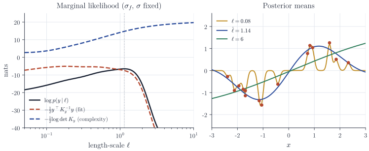
The marginal likelihood is generally not concave in the hyperparameters, and with few data it can have several local maxima, for instance one explaining the data as a slowly varying function with large noise and another as a rapidly varying function with small noise. Multiple restarts are prudent, and a fully Bayesian treatment places a prior on \(\gamma\) and integrates it out, usually by Markov chain Monte Carlo.

Remarks

The connection with kernel ridge regression goes further than the posterior mean. When the reproducing kernel Hilbert space \(\mathcal H\) of \(k\) is infinite-dimensional, sample paths of \(\mathcal{GP}(0,k)\) lie outside \(\mathcal H\) with probability one (under mild separability conditions this follows from Kallianpur’s zero–one law, since \(\mathcal H\) is the Cameron–Martin space of the prior), so the prior is not a distribution on the space in which the ridge estimator lives. The posterior standard deviation nevertheless has a deterministic meaning: in the noise-free case, \(\sqrt{k_{\mathrm{post}}(x,x)}\) is the worst-case error at \(x\) of the interpolant over the unit ball of \(\mathcal H\). Kanagawa, Hennig, Sejdinovic and Sriperumbudur, Gaussian processes and kernel methods: a review on connections and equivalences (2018), treat these links in detail. The standard reference for the material of this note is Rasmussen and Williams, Gaussian Processes for Machine Learning (2006), Chapters 2 and 5. The cubic cost of the Cholesky factorization is the main practical limitation; low-rank inducing-point approximations reduce it to \(O(nm^2)\) for \(m\) inducing inputs.