One posterior, four computations: grid, Laplace, Metropolis and variational inference

Once a model and a prior are written down, the posterior is determined; what remains is computation, and the choice of computational method changes what one actually reports. Below, the main options are applied to a single example in which the exact answer is available, so that each approximation can be compared with the truth. Three facts account for the differences that appear: the Laplace approximation is a second-order Taylor expansion at the mode, the Metropolis algorithm targets the posterior because its kernel satisfies detailed balance, and mean-field variational inference underestimates marginal variances when the parameters are correlated.

The example

We observe $n = 25$ pairs $(x_i, y_i)$ with $x_i$ drawn uniformly on $[0, 3]$ and

\[y_i \mid x_i \sim \mathrm{Bernoulli}\bigl(\sigma(\alpha + \beta x_i)\bigr), \qquad \sigma(t) = \frac{1}{1 + e^{-t}},\]

with independent $N(0, 2.5^2)$ priors on the intercept $\alpha$ and slope $\beta$. Write $\theta = (\alpha, \beta)$, $\ell(\theta) = \sum_i \{y_i \log\sigma(\eta_i) + (1 - y_i)\log\sigma(-\eta_i)\}$ with $\eta_i = \alpha + \beta x_i$, and

\[\log p(\theta \mid y) = \ell(\theta) - \frac{\norm{\theta}^2}{2 \cdot 2.5^2} - \log p(y),\]

where $p(y) = \int e^{\ell(\theta)}\pi(\theta)\,\dd\theta$ is the marginal likelihood. Since the covariates are all positive, the intercept and slope trade off against each other, and the posterior has strong negative correlation, about $-0.85$ in the simulated data set. That correlation is what separates the methods.

Point estimates

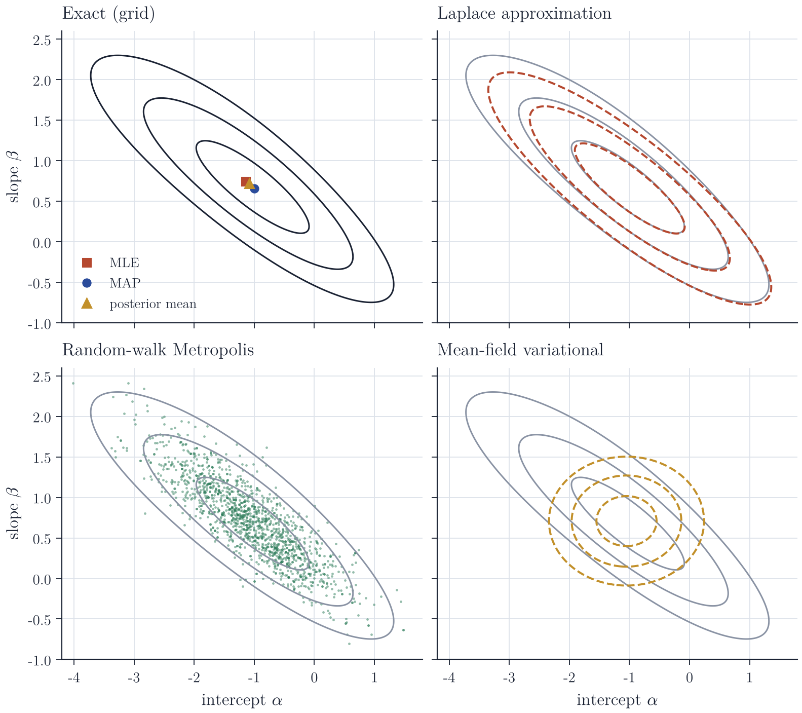
The maximum likelihood estimate maximizes $\ell$; the maximum a posteriori (MAP) estimate maximizes $\log p(\theta \mid y)$, which here is $\ell$ minus a ridge penalty, and it is pulled slightly towards zero. For the simulated data the MLE is $(-1.14, 0.74)$, the MAP estimate is $(-0.99, 0.66)$, and the posterior mean is $(-1.08, 0.72)$. The MAP estimate is a feature of a density, and densities are not invariant under reparametrization: if $\phi = g(\theta)$ for a smooth bijection $g$, the posterior density of $\phi$ carries the Jacobian factor $\lvert\det Dg^{-1}(\phi)\rvert$, which moves the mode. The posterior mean and quantiles of a fixed function of $\theta$ do not have this problem, but they require integrals, and integration is where the computational difficulty lies.

Exact computation on a grid

In two dimensions, the posterior can be computed by brute force: evaluate the unnormalized log density on a fine grid, exponentiate after subtracting the maximum, and normalize by a Riemann sum. With a $501 \times 501$ grid over a box containing essentially all the mass, this gives the reference answer in Figure 1, with posterior standard deviations $0.81$ for $\alpha$ and $0.50$ for $\beta$. The cost grows like $m^d$ for $m$ points per coordinate in dimension $d$, so the method is limited to a handful of parameters. The other three methods scale better, at the price of approximation error of different kinds.

The Laplace approximation

Let $\hat\theta$ be the MAP estimate and $H = -\nabla^2 \log p(\hat\theta \mid y)$, assumed positive definite. A second-order Taylor expansion at the mode, where the gradient vanishes, gives

\[\log p(\theta \mid y) \approx \log p(\hat\theta \mid y) - \tfrac12(\theta - \hat\theta)^\top H(\theta - \hat\theta),\]

so the posterior is approximated by $N(\hat\theta, H^{-1})$. Integrating the exponential of the same expansion approximates the marginal likelihood, $p(y) \approx e^{\ell(\hat\theta)}\pi(\hat\theta)(2\pi)^{d/2}\det(H)^{-1/2}$. The approximation is exact for Gaussian posteriors. For smooth models with a fixed number of parameters, the log posterior becomes increasingly quadratic on the scale $n^{-1/2}$ that matters, and under regularity conditions the relative error of the marginal likelihood approximation is of order $n^{-1}$ (Tierney and Kadane, 1986, Journal of the American Statistical Association). Here the logistic log likelihood is close to quadratic already: the Laplace standard deviations are $0.78$ and $0.47$, slightly smaller than the exact values, and the approximation is centred at the mode rather than at the mean, so it misses the mild skewness visible in the outer contours.

Markov chain Monte Carlo

The random-walk Metropolis algorithm generates a Markov chain $\theta^{(0)}, \theta^{(1)}, \dots$ as follows. Given $\theta^{(t)}$, draw a proposal $\theta' = \theta^{(t)} + \varepsilon$ with $\varepsilon \sim N(0, \Sigma)$, and set $\theta^{(t+1)} = \theta'$ with probability

\[a(\theta^{(t)}, \theta') = \min\Bigl\{1, \frac{p(\theta' \mid y)}{p(\theta^{(t)} \mid y)}\Bigr\},\]

and $\theta^{(t+1)} = \theta^{(t)}$ otherwise. Only ratios of the posterior density appear, so $p(y)$ is never needed.

Proposition 1. Let $p$ be a probability density on $\R^d$ that is positive everywhere, and let the proposal density $q(\theta, \theta')$ be symmetric, $q(\theta, \theta') = q(\theta', \theta)$. Then the Metropolis transition kernel leaves $p$ invariant: if $\theta^{(t)} \sim p$, then $\theta^{(t+1)} \sim p$.

Proof. The kernel is $K(\theta, \dd\theta') = q(\theta, \theta')a(\theta, \theta')\,\dd\theta' + r(\theta)\,\delta_\theta(\dd\theta')$, where $r(\theta) = 1 - \int q(\theta, u)a(\theta, u)\,\dd u$ is the rejection probability. For $\theta \ne \theta'$, symmetry of $q$ and the identity $p(\theta)\min\{1, p(\theta')/p(\theta)\} = \min\{p(\theta), p(\theta')\}$ give detailed balance,

\[p(\theta)\,q(\theta, \theta')\,a(\theta, \theta') = q(\theta, \theta')\min\{p(\theta), p(\theta')\} = p(\theta')\,q(\theta', \theta)\,a(\theta', \theta).\]

For a Borel set $A$, using detailed balance and then Fubini’s theorem (all integrands are nonnegative),

\[\begin{aligned} \int p(\theta) K(\theta, A)\,\dd\theta &= \int_A \int p(\theta') q(\theta', \theta) a(\theta', \theta)\,\dd\theta\,\dd\theta' + \int_A p(\theta) r(\theta)\,\dd\theta \\ &= \int_A p(\theta')\bigl(1 - r(\theta')\bigr)\dd\theta' + \int_A p(\theta) r(\theta)\,\dd\theta = \int_A p(\theta')\,\dd\theta'. \end{aligned}\]

Invariance alone does not guarantee convergence from an arbitrary starting point. With a Gaussian proposal and a positive continuous target the chain is irreducible with respect to Lebesgue measure and aperiodic, and an irreducible Metropolis–Hastings chain is also Harris recurrent (Tierney, 1994, Annals of Statistics). The distribution of $\theta^{(t)}$ then converges to $p$ in total variation from every starting point, and averages $T^{-1}\sum_{t \le T} f(\theta^{(t)})$ converge almost surely to $\int f p$ for every $p$-integrable $f$ (see also Robert and Casella, Monte Carlo Statistical Methods). How fast this happens depends on the proposal, and a proposal shaped like the posterior helps most. We use $\Sigma = (2.38^2/d)H^{-1}$: the Laplace covariance supplies the shape, and the factor $2.38^2/d$ comes from the optimal-scaling analysis of Roberts, Gelman and Gilks (1997, Annals of Applied Probability). That analysis is asymptotic in the dimension $d$, so in two dimensions it is only a reasonable default. The chain accepts 37% of proposals, and after discarding 2,000 of 20,000 iterations its sample standard deviations are $0.80$ and $0.49$, within Monte Carlo error of the exact values. The price is computing time: the draws are positively autocorrelated, and the 18,000 retained draws have an estimated effective sample size of about 2,500 for each coordinate, so every posterior summary carries a Monte Carlo error that has to be estimated.

Variational inference

Variational inference replaces integration by optimization. For any probability density $q$ on $\R^d$ that is absolutely continuous with respect to the posterior and for which the expectations below are finite, define the evidence lower bound

\[\mathrm{ELBO}(q) = \E_q\bigl[\ell(\theta) + \log\pi(\theta)\bigr] - \E_q[\log q(\theta)].\]

Proposition 2. $\log p(y) = \mathrm{ELBO}(q) + \KL\bigl(q \,\Vert\, p(\cdot \mid y)\bigr)$. In particular $\mathrm{ELBO}(q) \le \log p(y)$, and maximizing the ELBO over a family of densities is the same as minimizing $\KL(q \,\Vert\, p(\cdot \mid y))$ over that family.

Proof. Substitute $\log p(\theta \mid y) = \ell(\theta) + \log\pi(\theta) - \log p(y)$ into $\KL(q \,\Vert\, p(\cdot \mid y)) = \E_q[\log q(\theta) - \log p(\theta \mid y)]$ and rearrange. Nonnegativity of the Kullback–Leibler divergence gives the inequality.

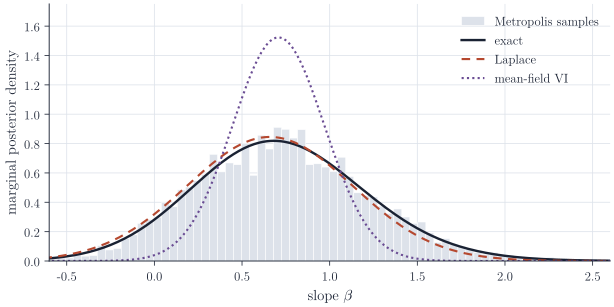
The mean-field Gaussian family takes $q(\theta) = N(\alpha; m_1, s_1^2)\,N(\beta; m_2, s_2^2)$, with independent coordinates. Its entropy is $\log s_1 + \log s_2$ plus a constant, and the expected log posterior can be computed by two-dimensional Gauss–Hermite quadrature, so the ELBO is a smooth function of four numbers that a standard optimizer maximizes. The result is centred well, with means $(-1.05, 0.71)$, but its standard deviations are $0.43$ and $0.26$, about half the exact values (Figures 1 and 2). The optimizer has converged; the shrinkage is a property of the optimal member of the mean-field family when the target is correlated, and the Gaussian case can be solved exactly.

Proposition 3. Let the target be $N(\mu, \Sigma)$ on $\R^d$ with precision matrix $\Lambda = \Sigma^{-1}$. Among product densities $q = \prod_{i} N(m_i, s_i^2)$, the Kullback–Leibler divergence $\KL(q \,\Vert\, N(\mu, \Sigma))$ is minimized by $m = \mu$ and $s_i^2 = 1/\Lambda_{ii}$. Moreover $1/\Lambda_{ii} \le \Sigma_{ii}$, with equality for all $i$ if and only if $\Sigma$ is diagonal.

Proof. With $S = \diag(s_1^2, \dots, s_d^2)$, the divergence between Gaussians is

\[\KL\bigl(N(m, S) \,\Vert\, N(\mu, \Sigma)\bigr) = \frac12\Bigl\{\tr(\Lambda S) + (m - \mu)^\top\Lambda(m - \mu) - d - \log\det S + \log\det\Sigma\Bigr\}.\]

The term in $m$ is minimized at $m = \mu$ because $\Lambda$ is positive definite. The rest separates over coordinates as $\frac12\sum_i (\Lambda_{ii}s_i^2 - \log s_i^2)$ plus a constant, and $u \mapsto \Lambda_{ii}u - \log u$ is strictly convex on $(0, \infty)$ with minimum at $u = 1/\Lambda_{ii}$. For the inequality, write $e_i$ for the $i$th unit vector and apply the Cauchy–Schwarz inequality to $\Sigma^{1/2}e_i$ and $\Sigma^{-1/2}e_i$:

\[1 = (e_i^\top e_i)^2 = \bigl((\Sigma^{1/2}e_i)^\top(\Sigma^{-1/2}e_i)\bigr)^2 \le (e_i^\top\Sigma e_i)(e_i^\top\Sigma^{-1}e_i) = \Sigma_{ii}\Lambda_{ii},\]

with equality if and only if $\Sigma^{1/2}e_i$ and $\Sigma^{-1/2}e_i$ are parallel, that is, if and only if $e_i$ is an eigenvector of $\Sigma$. This holds for every $i$ exactly when $\Sigma$ is diagonal.

In two dimensions with correlation $\rho$, $1/\Lambda_{ii} = \Sigma_{ii}(1 - \rho^2)$, the conditional variance of one coordinate given the other. The mean-field approximation therefore reports conditional spreads as if they were marginal ones, and the standard deviations shrink by the factor $\sqrt{1 - \rho^2}$, about $0.53$ for $\rho = -0.85$, which is close to what the logistic example shows. The direction of the divergence matters as well: $\KL(q \,\Vert\, p)$ penalizes $q$ heavily for putting mass where $p$ has little, and only mildly for missing mass that $p$ has, so the optimal $q$ fits inside the posterior.

Marginal posterior density of the slope: exact curve, Laplace approximation, histogram of Metropolis draws and a much narrower mean-field variational density — Figure 2. Marginal posterior of the slope $\beta$. The Laplace approximation and the Metropolis histogram agree closely with the exact density; the mean-field variational density has roughly half the exact standard deviation.

Remarks

The guarantees differ in kind. The grid error is a discretization error and the MCMC error is a Monte Carlo error; both can be driven to zero with more computation. The Laplace and variational errors are approximation errors of a fixed family and do not decrease with computing time. The Laplace approximation is accurate when the posterior is close to Gaussian, which the Bernstein–von Mises theorem makes likely in regular parametric models with many observations, and it degrades for skewed, multimodal or constrained posteriors. A factorized variational family understates marginal uncertainty whenever the posterior is correlated, often while getting the means nearly right; richer families (a full-covariance Gaussian, or the parameter blocks of a structured mean-field approximation) reduce or remove the effect at higher cost. Blei, Kucukelbir and McAuliffe (2017, Journal of the American Statistical Association) review variational methods from a statistical point of view, and Gelman and coauthors, Bayesian Data Analysis, treat the Laplace approximation and MCMC in applied settings.