Fitting the wrong model by maximum likelihood: Kullback–Leibler projections and sandwich standard errors

October 12, 2026Statistical theory

Every parametric model is an approximation, so the useful question about maximum likelihood is what it does when the data are generated by a law \(P\) outside the model \(\{P_\theta : \theta \in \Theta\}\). Two separate things change. The estimator converges to a well-defined parameter \(\theta^*\), but \(\theta^*\) is determined jointly by the model and by \(P\), and it need not have the interpretation the model suggests. And the asymptotic variance of the estimator is no longer the inverse Fisher information, so standard errors computed from the model are inconsistent. Both points can be made precise with short arguments, and two simple models show how much they matter.

Throughout, \(X_1, X_2, \dots\) are i.i.d. with law \(P\), which has density \(p\) with respect to a \(\sigma\)-finite measure \(\mu\); the model densities \(p_\theta\) are with respect to the same \(\mu\); and \(\hat\theta_n\) maximizes \(\ell_n(\theta) = \sum_{i=1}^n \log p_\theta(X_i)\).

What is being estimated

If \(\E_P \abs{\log p(X)} < \infty\) and \(\E_P \abs{\log p_\theta(X)} < \infty\), then

\[\E_P \log p_\theta(X) = \E_P \log p(X) - \KL(P \,\Vert\, P_\theta).\]

The first term does not depend on \(\theta\), so maximizing the expected log-likelihood is the same as minimizing the Kullback–Leibler divergence from \(P\) to the model. The natural target is therefore

\[\theta^* = \argmin_{\theta \in \Theta} \KL(P \,\Vert\, P_\theta),\]

the Kullback–Leibler projection of \(P\) onto the model, assumed to exist and to be unique. When \(P = P_{\theta_0}\) belongs to an identifiable model, \(\theta^* = \theta_0\). Wald’s argument for consistency uses nothing about the model beyond the integrability of envelope functions under the law that generates the data. Repeating it with \(m_\theta = \log(p_\theta / p_{\theta^*})\) in place of the log-likelihood ratio relative to the true parameter, and with uniqueness of \(\theta^*\) in place of identifiability, shows \(\hat\theta_n \to \theta^*\) almost surely under the corresponding conditions.

Which member of the model is closest to \(P\) depends on the divergence, and the Kullback–Leibler divergence weighs the discrepancy by \(P\). Two examples make this concrete.

Exponential families match moments. Let \(p_\theta(x) = h(x) \exp\bigl(\theta^\top T(x) - A(\theta)\bigr)\) be a minimal canonical exponential family with open natural parameter space \(\Theta \subseteq \R^k\). Then \(A\) is infinitely differentiable and strictly convex on \(\Theta\), with \(\nabla A(\theta) = \E_\theta T(X)\).

Proposition 1. Suppose \(\E_P \lVert T(X) \rVert < \infty\), \(\E_P \abs{\log h(X)} < \infty\), and there is \(\theta^* \in \Theta\) with \(\E_{\theta^*} T(X) = \E_P T(X)\). Then \(\theta^*\) is the unique maximizer of \(\theta \mapsto \E_P \log p_\theta(X)\) over \(\Theta\).

Proof. Write \(\tau = \E_P T(X)\). By the integrability assumptions,

\[\E_P \log p_\theta(X) = \E_P \log h(X) + \theta^\top \tau - A(\theta),\]

which is a strictly concave differentiable function of \(\theta\) with gradient \(\tau - \nabla A(\theta)\). The gradient vanishes at \(\theta^*\). A stationary point of a differentiable concave function is a global maximizer, and strict concavity makes it unique.

So fitting a normal distribution by maximum likelihood matches the mean and variance of \(P\), whatever the shape of \(P\); fitting an exponential distribution matches the mean; fitting a Poisson distribution matches the mean and ignores the variance. The sample version is the familiar likelihood equation \(\nabla A(\hat\theta_n) = n^{-1} \sum_i T(X_i)\).

Normal linear regression estimates the best linear predictor. Suppose pairs \((Z_i, Y_i)\) are i.i.d. with \(\E \lVert Z \rVert^2 < \infty\), \(\E Y^2 < \infty\) and \(\E ZZ^\top\) nonsingular, and the working model says \(Y \mid Z \sim N(Z^\top \beta, \sigma^2)\). The expected conditional log-likelihood is

\[-\tfrac12 \log(2\pi\sigma^2) - \frac{\E(Y - Z^\top \beta)^2}{2\sigma^2},\]

maximized by \(\beta^* = (\E ZZ^\top)^{-1} \E ZY\) and \(\sigma^{*2} = \E(Y - Z^\top \beta^*)^2\). The target is the population least-squares coefficient. If the regression function \(m(z) = \E(Y \mid Z = z)\) is not linear, \(\beta^*\) is the linear approximation to \(m\) that is best in \(L^2(P_Z)\), and it changes with the distribution of the covariates.

Figure 1. The same conditional law, $Y = 2\sin Z + \varepsilon$ with $\varepsilon \sim N(0, 0.5^2)$, under two covariate distributions (shaded densities). The population slope is $\beta_1^* = \mathrm{Cov}(Z, m(Z))/\mathrm{Var}(Z) = \mathrm{E}\, m'(Z) = 2\cos(\mu_Z) e^{-\sigma_Z^2/2}$ by Stein's lemma, so it is $1.21$ under design A and $0.12$ under design B. Dashed: the least-squares fit to $300$ observations.

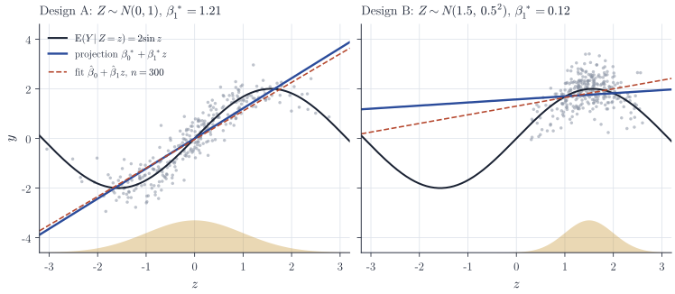
Both slopes in Figure 1 are correct answers to the question the model asks, and neither describes the regression function well. The sandwich variance below gives honest uncertainty for \(\hat\beta\) as an estimator of \(\beta^*\); it does not make \(\beta^*\) more meaningful.

The limiting distribution

Write \(s_\theta(x) = \nabla_\theta \log p_\theta(x)\) for the score and define

\[J = -\E_P \nabla^2_\theta \log p_{\theta^*}(X), \qquad K = \E_P\, s_{\theta^*}(X) s_{\theta^*}(X)^\top .\]

Theorem 2. Let \(\theta^*\) be an interior point of \(\Theta \subseteq \R^k\) and the unique maximizer of \(\E_P \log p_\theta(X)\). Assume that \(\hat\theta_n \xrightarrow{p} \theta^*\), that \(\sum_i s_{\hat\theta_n}(X_i) = 0\) with probability tending to one, and that

1. on a closed ball \(U\) around \(\theta^*\), contained in the interior of \(\Theta\), \(\E_P \abs{\log p_\theta(X)} < \infty\) for each \(\theta \in U\), \(\theta \mapsto \log p_\theta(x)\) is twice continuously differentiable for every \(x\), with \(\sup_{\theta \in U} \lVert \nabla^2_\theta \log p_\theta(x) \rVert \le m(x)\) and \(\E_P\, m(X) < \infty\);
2. \(\E_P \lVert s_{\theta^*}(X) \rVert^2 < \infty\) and \(J\) is nonsingular.

Then \(\sqrt n (\hat\theta_n - \theta^*) \rightsquigarrow N_k\bigl(0, J^{-1} K J^{-1}\bigr)\).

Proof. First, \(\E_P\, s_{\theta^*}(X) = 0\). For \(\theta \in U\) and every \(x\), the mean value inequality gives \(\lVert s_\theta(x) \rVert \le \lVert s_{\theta^*}(x) \rVert + r\, m(x)\), where \(r\) is the radius of \(U\); the right-hand side is integrable. Hence the difference quotients of \(\theta \mapsto \log p_\theta(x)\) are dominated by an integrable function on \(U\), dominated convergence gives \(\nabla_\theta \E_P \log p_\theta(X) = \E_P\, s_\theta(X)\) on the interior of \(U\), and this gradient vanishes at the interior maximizer \(\theta^*\).

The estimator is then a Z-estimator with estimating function \(\psi(x, \theta) = s_\theta(x)\), for which \(\E_P\, \dot\psi(X, \theta^*) = -J\) and \(\E_P\, \psi \psi^\top = K\). The one-term expansion of the estimating equation, controlled by the local domination in condition 1, gives

\[\sqrt n (\hat\theta_n - \theta^*) = J^{-1} \frac{1}{\sqrt n} \sum_{i=1}^n s_{\theta^*}(X_i) + o_P(1),\]

and the multivariate central limit theorem finishes the proof. The details of the expansion are the same as for general M-estimators; see the note on M-estimators.

Under correct specification \(P = P_{\theta_0}\), differentiating \(\int p_\theta \, \dd\mu = 1\) twice under the integral sign (which requires its own domination condition on the first two derivatives of \(p_\theta\)) gives the information identity \(K = J = I(\theta_0)\), and the covariance collapses to \(I(\theta_0)^{-1}\). Nothing forces \(K = J\) when \(P\) is outside the model. Standard errors computed from the observed or expected information estimate \(J^{-1}\), which is the wrong matrix; the plug-in estimator \(\hat J^{-1} \hat K \hat J^{-1}\), with \(\hat J = -n^{-1} \sum_i \nabla^2 \log p_{\hat\theta_n}(X_i)\) and \(\hat K = n^{-1} \sum_i s_{\hat\theta_n}(X_i) s_{\hat\theta_n}(X_i)^\top\), is consistent for the right one under mild additional domination. The discrepancy between \(\hat J\) and \(\hat K\) is itself informative and is the basis of White’s information matrix test for misspecification.

Two calculations

Exponential model, positive data. Fit \(p_\lambda(x) = \lambda e^{-\lambda x}\), \(x > 0\), to i.i.d. positive data with mean \(m\) and variance \(v\). Then \(\E_P \log p_\lambda(X) = \log \lambda - \lambda m\), so \(\lambda^* = 1/m\) (Proposition 1 with \(T(x) = -x\)), and \(\hat\lambda_n = 1/\bar X_n\). The score is \(1/\lambda - x\), so

\[J = \frac{1}{\lambda^{*2}} = m^2, \qquad K = \Var_P(X) = v, \qquad J^{-1} K J^{-1} = \frac{v}{m^4} = \lambda^{*2} \cdot \frac{v}{m^2}.\]

The model-based variance is \(J^{-1} = \lambda^{*2}\). The ratio of the true to the model-based asymptotic variance is the squared coefficient of variation \(\mathrm{CV}^2 = v/m^2\), which equals \(1\) for exponential data, as it must. Because \(\sqrt n(\hat\lambda_n - \lambda^*)/\hat\lambda_n \rightsquigarrow N(0, \mathrm{CV}^2)\), the nominal \(95\%\) interval \(\hat\lambda_n \pm 1.96\, \hat\lambda_n / \sqrt n\) has asymptotic coverage

\[\P\bigl(\abs{N(0, \mathrm{CV}^2)} \le 1.96\bigr) = 2\Phi(1.96/\mathrm{CV}) - 1 .\]

For log-normal data with shape \(s\), \(\mathrm{CV}^2 = e^{s^2} - 1\). The interval is conservative when \(s < \sqrt{\log 2} \approx 0.83\) and anti-conservative beyond, with coverage below \(0.5\) by \(s = 1.6\). The sandwich interval \(\hat\lambda_n \pm 1.96\, \hat v_n^{1/2} / (\sqrt n\, \bar X_n^2)\), where \(\hat v_n\) is the sample variance, has asymptotic coverage \(0.95\) for every \(s\).

Figure 2. Exponential model fitted to log-normal data with shape $s$. Coverage of nominal $95\%$ Wald intervals for $\lambda^* = 1/\mathrm{E}X$ based on the model variance $\hat\lambda^2/n$ (red) and on the sandwich (blue). Lines: asymptotic coverage. Points: $20{,}000$ replications at $n = 100$ (circles) and $n = 1000$ (squares).

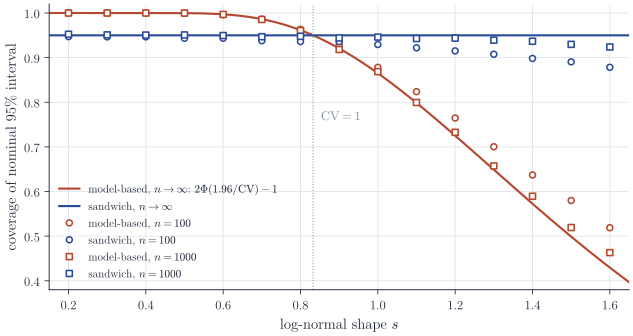
Figure 2 also shows the price of robustness. The sandwich needs a good estimate of \(\Var_P(X)\), and for large \(s\) the log-normal is so skewed that the sample variance is unreliable even at \(n = 1000\); coverage approaches \(0.95\) slowly. The model-based interval converges quickly, to the wrong answer.

Linear regression. In the regression example, \(J\) is block diagonal in \((\beta, \sigma^2)\) because the normal equations give \(\E Z\varepsilon = 0\) for \(\varepsilon = Y - Z^\top \beta^*\). The \(\beta\)-block of the sandwich is

\[(\E ZZ^\top)^{-1}\, \E\bigl[\varepsilon^2 ZZ^\top\bigr]\, (\E ZZ^\top)^{-1},\]

which is the population version of the heteroskedasticity-consistent covariance of Eicker, Huber and White, while the model-based covariance is \(\sigma^{*2} (\E ZZ^\top)^{-1}\). The decomposition

\[\varepsilon = \bigl(m(Z) - Z^\top \beta^*\bigr) + \bigl(Y - m(Z)\bigr)\]

shows what is needed for the two to agree: \(\E[\varepsilon^2 ZZ^\top] = \E[\varepsilon^2]\, \E[ZZ^\top]\), which holds when \(\E[\varepsilon^2 \mid Z]\) is constant. A nonlinear \(m\) makes the squared approximation error depend on \(Z\), so it acts exactly like heteroskedasticity even when \(\Var(Y \mid Z)\) is constant. In design B of Figure 1 the approximation error is small where the covariates concentrate and large in the tails of \(P_Z\).

Remarks

Misspecification does not always move the target. If a generalized linear model has the correct mean function but the wrong variance function, for instance Poisson regression applied to overdispersed counts with \(\E(Y \mid Z) = \exp(Z^\top \beta_0)\), the expected score \(\E\bigl[Z(Y - \exp(Z^\top \beta))\bigr]\) vanishes at \(\beta = \beta_0\), so \(\theta^* = \beta_0\) and only the standard errors need repair. This is the starting point of quasi-likelihood and of generalized estimating equations. In general, the sandwich protects the variance, but whether \(\theta^*\) answers the scientific question has to be argued separately.

Classical references are P. J. Huber, “The behavior of maximum likelihood estimates under nonstandard conditions” (Fifth Berkeley Symposium, 1967), and H. White, “Maximum likelihood estimation of misspecified models”, Econometrica (1982). D. A. Freedman, “On the so-called ‘Huber sandwich estimator’ and ‘robust standard errors’”, The American Statistician (2006), argues the caveat of the previous paragraph forcefully, and A. Buja and coauthors, “Models as approximations I”, Statistical Science (2019), develop the regression case in detail.