Learning the prior from many parallel problems: empirical Bayes for normal means
The choice of prior is usually described as an act of judgement made before the data arrive. Empirical Bayes methods take a different view in one particular situation: when the data consist of many parallel problems of the same kind, such as the effects of thousands of genes, the batting records of many players or the outcomes in many hospitals, the collection of problems carries information about the distribution from which the individual parameters were drawn. That distribution plays the role of the prior, and it can be estimated. Robbins (1956, Proceedings of the Third Berkeley Symposium) introduced the idea; Efron and Morris (1973, Journal of the American Statistical Association) showed that it explains the James–Stein estimator.
The normal means problem
Throughout, \(\theta = (\theta_1, \dots, \theta_p)\) is unknown and we observe
\[X_i \mid \theta \sim N(\theta_i, 1), \qquad i = 1, \dots, p, \quad \text{independently}.\]The loss is \(\norm{\hat\theta - \theta}^2\). The maximum likelihood estimator \(\hat\theta^{\mathrm{ML}} = X\) has risk \(\E_\theta\norm{X - \theta}^2 = p\) for every \(\theta\).
Suppose now that \(\theta_1, \dots, \theta_p\) are themselves independent draws from a distribution \(G\). The Bayes rule under squared error is the posterior mean \(\E[\theta_i \mid X_i]\), which depends on \(G\). If \(G\) were known we would use it. It is not known, but the \(X_i\) are independent with common marginal density
\[f(x) = \int \varphi(x - t) \, G(\dd t),\]where \(\varphi\) is the standard normal density. With \(p\) large, \(f\) can be estimated well from \(X_1, \dots, X_p\), and through \(f\) we learn about \(G\). The other coordinates act as a sample from the prior of each one.
Linear empirical Bayes and the James–Stein estimator
Take first a normal prior \(G = N(0, A)\) with unknown \(A > 0\). Then \(\theta_i \mid X_i \sim N\bigl((1 - B)X_i, 1 - B\bigr)\) with \(B = 1/(1 + A)\), so the Bayes rule shrinks each coordinate towards zero by the factor \(1 - B\). Marginally the \(X_i\) are independent \(N(0, 1 + A)\), so \(S = \norm{X}^2\) satisfies \(S/(1 + A) \sim \chi^2_p\). For \(p \ge 3\) the chi-squared density gives
\[\E\Bigl[\frac{1}{\chi^2_p}\Bigr] = \frac{\int_0^\infty x^{p/2 - 2} e^{-x/2}\,\dd x}{2^{p/2}\Gamma(p/2)} = \frac{2^{p/2-1}\Gamma(p/2 - 1)}{2^{p/2}\Gamma(p/2)} = \frac{1}{p - 2},\]hence \(\E[(p-2)/S] = 1/(1 + A) = B\): the statistic \((p-2)/S\) is an unbiased estimator of the shrinkage factor. Plugging it into the Bayes rule gives the James–Stein estimator
\[\hat\theta^{\mathrm{JS}} = \Bigl(1 - \frac{p - 2}{\norm{X}^2}\Bigr) X .\]The derivation used the normal prior. The conclusion does not need it.
Theorem 1 (James–Stein). Let \(p \ge 3\). For every \(\theta \in \R^p\),
\[\E_\theta \norm{\hat\theta^{\mathrm{JS}} - \theta}^2 = p - (p-2)^2 \, \E_\theta\Bigl[\frac{1}{\norm{X}^2}\Bigr] < p .\]The proof rests on Stein’s identity: if \(Z \sim N(\mu, 1)\) and \(h : \R \to \R\) is absolutely continuous with \(\E\abs{h'(Z)} < \infty\), then \(\E[(Z - \mu)h(Z)] = \E[h'(Z)]\). It is integration by parts, using \(\varphi'(z) = -z\varphi(z)\); a proof free of boundary terms writes \(\E[(Z - \mu)h(Z)] = \E[(Z - \mu)(h(Z) - h(\mu))]\), substitutes \(h(z) - h(\mu) = \int_\mu^z h'(v)\,\dd v\), exchanges the order of integration by Fubini’s theorem, which \(\E\abs{h'(Z)} < \infty\) permits, and uses \(\int_v^\infty (z - \mu)\varphi(z - \mu)\,\dd z = \varphi(v - \mu)\) for \(v > \mu\) and the mirror identity for \(v < \mu\) (Stein, 1981, Annals of Statistics).
Proof. Write \(g_i(x) = x_i/\norm{x}^2\). Expanding the square,
\[\norm{\hat\theta^{\mathrm{JS}} - \theta}^2 = \norm{X - \theta}^2 - 2(p - 2)\sum_{i=1}^p (X_i - \theta_i)\, g_i(X) + \frac{(p - 2)^2}{\norm{X}^2}.\]The first term has expectation \(p\). For the last, \(\E_\theta\norm{X}^{-2} < \infty\) when \(p \ge 3\): near the origin the density of \(X\) is bounded and \(\int_{\norm{x} \le 1} \norm{x}^{-2}\,\dd x < \infty\) in dimension \(p \ge 3\). For the middle term, fix \(i\) and the coordinates \(X_j\), \(j \ne i\); for almost every value of these (all except the null event that they all vanish), \(x_i \mapsto g_i(x)\) is smooth with
\[\partial_i g_i(x) = \frac{1}{\norm{x}^2} - \frac{2x_i^2}{\norm{x}^4}, \qquad \abs{\partial_i g_i(x)} \le \frac{3}{\norm{x}^2}.\]Applying Stein’s identity conditionally on \((X_j)_{j \ne i}\), which is legitimate by independence of the coordinates and the integrability just shown, and then summing over \(i\),
\[\E_\theta \sum_{i=1}^p (X_i - \theta_i)\, g_i(X) = \E_\theta \sum_{i=1}^p \partial_i g_i(X) = \E_\theta\Bigl[\frac{p}{\norm{X}^2} - \frac{2}{\norm{X}^2}\Bigr] = (p-2)\, \E_\theta\Bigl[\frac{1}{\norm{X}^2}\Bigr].\]Combining the three terms gives the risk formula. The expectation \(\E_\theta\norm{X}^{-2}\) is strictly positive, so the risk is strictly less than \(p\).
So an argument that began with a Bayesian model for \(\theta\) has produced an estimator that dominates the maximum likelihood estimator in the strict frequentist sense, uniformly over the parameter space. The improvement is largest when \(\norm{\theta}\) is small relative to \(\sqrt p\), which is when the empirical Bayes picture of a concentrated prior near zero is accurate; for large \(\norm\theta\) the risk approaches \(p\) from below. In practice one shrinks towards the grand mean \(\bar X\) instead of zero, which costs one degree of freedom: \(\hat\theta_i = \bar X + \bigl(1 - (p-3)/\sum_j (X_j - \bar X)^2\bigr)(X_i - \bar X)\), valid for \(p \ge 4\), usually with the factor truncated at zero (the positive-part estimator, which has smaller risk still).
Without a parametric prior: Tweedie’s formula
A normal prior is convenient but often wrong. Many large-scale problems have mostly null effects and a minority of real ones, and a normal \(G\) shrinks both groups by the same factor. Remarkably, the posterior mean can be written in terms of the marginal density alone.
Proposition 2 (Tweedie’s formula). Let \(\theta \sim G\), an arbitrary probability distribution on \(\R\), and \(X \mid \theta \sim N(\theta, 1)\). Then \(f\) is strictly positive and differentiable on \(\R\), and for every \(x\)
\[\E[\theta \mid X = x] = x + \frac{f'(x)}{f(x)} = x + \frac{\dd}{\dd x}\log f(x).\]Proof. Positivity is clear since \(\varphi > 0\). For differentiation under the integral sign, \(\partial_x \varphi(x - t) = -(x - t)\varphi(x - t)\) is bounded in absolute value by \(\sup_u \abs{u}\varphi(u) = (2\pi e)^{-1/2}\), a constant that is integrable against the probability measure \(G\). By the dominated convergence theorem (applied to difference quotients, using the mean value theorem),
\[f'(x) = -\int (x - t)\varphi(x - t) \, G(\dd t) = -x f(x) + \int t \, \varphi(x - t) \, G(\dd t).\]The last integral is finite for the same reason, and dividing by \(f(x)\) gives \(x + f'(x)/f(x) = \int t\,\varphi(x - t)\,G(\dd t)/f(x) = \E[\theta \mid X = x]\) by Bayes’ formula.
The formula requires no knowledge of \(G\) beyond what is encoded in \(f\), and \(f\) is the density of the observed data. An empirical Bayes estimator follows by estimating \(\log f\) smoothly and differentiating. A simple method, used by Efron (2011, Journal of the American Statistical Association) in his discussion of the formula, bins the \(X_i\) into a histogram and fits a Poisson regression of the bin counts on a polynomial in the bin centres. The fitted log-density is then a polynomial whose derivative is available in closed form. Proposition 2 has an analogue for every exponential family, stated for the natural parameter; for a \(N(\theta, \sigma^2)\) likelihood with known \(\sigma\) it reads \(\E[\theta \mid x] = x + \sigma^2 (\log f)'(x)\).
The formula also explains selection bias. If we report the coordinates with the largest \(X_i\), these are biased upwards as estimates of their \(\theta_i\), and the correction \((\log f)'(x)\) is negative in the right tail of \(f\), which shrinks exactly those coordinates back. The correction depends only on the data distribution, not on how the selection was made, because the posterior mean conditions on \(X_i = x\).
A comparison
We take \(p = 1000\) and a prior that is not normal,
\[G = 0.7\,\delta_0 + 0.3\,N(3, 0.5^2),\]so that 70% of the means are exactly zero and the rest cluster around \(3\). Figure 1 shows one data set. The left panel shows the marginal density and its estimate from a degree-5 log-polynomial fitted to a 60-bin histogram. The right panel compares the estimated rules with the oracle posterior mean under the true \(G\), which is available in closed form for this mixture.
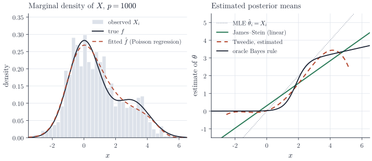
The oracle rule is far from linear. It sets small observations almost exactly to zero, since an observation near zero is most likely a null coordinate, and pulls observations near \(3\) towards the centre of the non-null cluster. The James–Stein rule can only choose a single slope, here about \(0.63\), which is a compromise between the two behaviours. Tweedie’s formula with the estimated \(f\) tracks the shape of the oracle rule over the bulk of the data.
Over 200 replications of the experiment, the average squared error per coordinate was \(1.00\) for the maximum likelihood estimator, \(0.66\) for positive-part James–Stein towards the grand mean, \(0.51\) for Tweedie’s formula with the estimated density, and \(0.43\) for the oracle Bayes rule. Most of the gap between linear shrinkage and the oracle is recovered without assuming anything about the form of \(G\).
Remarks
Empirical Bayes uses the data twice, once to choose the prior and once to compute posteriors, and naive posterior intervals that ignore the estimation of \(G\) are too narrow. Morris (1983, Journal of the American Statistical Association) discusses corrections in the parametric case; a fully Bayesian alternative places a hyperprior on the parameters of \(G\), which for large \(p\) gives similar point estimates and properly widened intervals. Instead of estimating \(f\) (the “f-modelling” route above), one can estimate \(G\) directly, for instance by the nonparametric maximum likelihood estimator of Kiefer and Wolfowitz (1956); Jiang and Zhang (2009, Annals of Statistics) show that the resulting empirical Bayes rule nearly attains the oracle risk in the normal means problem. Efron’s book Large-Scale Inference develops these ideas together with empirical Bayes approaches to false discovery rates.