Expectation–maximization as coordinate ascent on the evidence lower bound

The EM algorithm of Dempster, Laird and Rubin (Maximum likelihood from incomplete data via the EM algorithm, JRSS-B, 1977) is usually presented as an alternation between computing a conditional expectation and maximizing it. Neal and Hinton (A view of the EM algorithm that justifies incremental, sparse, and other variants, 1998) observed that both steps maximize a single functional of two arguments, a distribution over the latent variables and the parameter. That functional is the evidence lower bound of variational inference. The correspondence explains why EM increases the likelihood, which variants keep that property, and in what sense EM is variational inference with a point mass for the parameter; a one-parameter mixture shows how the convergence rate is tied to the fraction of missing information.

Setting

Data $x$ are observed, $z$ is latent, and $\theta \in \Theta \subseteq \R^k$ is a parameter. The complete-data model has density $p(x, z \mid \theta)$ with respect to a product of a fixed measure in $x$ and a $\sigma$-finite measure $\nu$ in $z$ (counting measure for discrete $z$). The likelihood is $p(x\mid\theta) = \int p(x, z\mid\theta)\, \nu(\dd z)$, assumed positive and finite, and $\ell(\theta) = \log p(x\mid\theta)$. The conditional density of $z$ is $p(z\mid x, \theta) = p(x,z\mid\theta)/p(x\mid\theta)$.

For a density $q$ on the latent space (with respect to $\nu$) define

\[F(q, \theta) = \E_q\bigl[\log p(x, Z\mid\theta)\bigr] + H(q), \qquad H(q) = -\E_q \log q(Z),\]

whenever both terms are finite. This is the ELBO of the approximation $q$ to $p(z\mid x,\theta)$.

Lemma 1. If $F(q, \theta)$ is defined, then $F(q, \theta) = \ell(\theta) - \mathrm{KL}\bigl(q\Vert p(\cdot\mid x, \theta)\bigr)$. In particular $F(q, \theta) \le \ell(\theta)$, with equality if and only if $q = p(\cdot \mid x, \theta)$ $\nu$-almost everywhere.

Proof. On $\{q > 0\}$, $\log p(x, z\mid\theta) - \log q(z) = \ell(\theta) - \log\bigl(q(z)/p(z\mid x, \theta)\bigr)$. Integrating against $q$ gives the identity, the integrals being finite because $F(q,\theta)$ is. The inequality and the equality case are those of the Kullback–Leibler divergence.

EM as coordinate ascent

Given a current value $\theta_t$, coordinate ascent on $F$ first maximizes over $q$ with $\theta = \theta_t$ and then over $\theta$ with $q$ fixed.

Proposition 2. Let $q_{t+1} = p(\cdot\mid x, \theta_t)$ and suppose $\theta_{t+1}$ maximizes $\theta \mapsto F(q_{t+1}, \theta)$ over $\Theta$. Then

$q_{t+1}$ maximizes $q \mapsto F(q, \theta_t)$ (the E-step);
$\theta_{t+1}$ maximizes $Q(\theta \mid \theta_t) = \E\bigl[\log p(x, Z \mid \theta) \mid x, \theta_t\bigr]$ (the M-step);
$\ell(\theta_{t+1}) \ge \ell(\theta_t)$.

Proof. Part 1 is the equality case of Lemma 1. For part 2, $F(q_{t+1}, \theta) = Q(\theta\mid\theta_t) + H(q_{t+1})$ and the entropy does not depend on $\theta$. For part 3, by Lemma 1 and the two maximizations,

\[\ell(\theta_{t+1}) \ge F(q_{t+1}, \theta_{t+1}) \ge F(q_{t+1}, \theta_t) = \ell(\theta_t).\]

The chain of inequalities in part 3 is the whole monotonicity argument, and it shows at once which modifications preserve it. The M-step need only increase $F(q_{t+1}, \cdot)$, which is generalized EM. The E-step need only increase $F(\cdot, \theta_t)$, which justifies updating the latent distribution for a subset of observations at a time; this was the motivation of Neal and Hinton. If $q$ is restricted to a family that does not contain $p(\cdot\mid x,\theta)$, coordinate ascent still increases $F$, but $F(q_t,\theta_t)$ now lies strictly below $\ell(\theta_t)$ and the fixed points are in general not stationary points of $\ell$. This is variational EM, and its bias is governed by the Kullback–Leibler gap in Lemma 1.

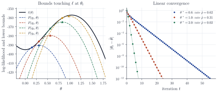
Figure 1 (left) shows the geometry: $\theta \mapsto F(q_{t+1}, \theta)$ is a minorant of $\ell$ that touches it at $\theta_t$, and the M-step moves to the top of the minorant.

Where the posterior of the parameter went

Now treat $\theta$ as random with prior density $p(\theta)$ and approximate the joint posterior of $(z, \theta)$ by a product $q(z)\,r(\theta)$. The ELBO is

\[\mathcal L(q, r) = \E_{q \otimes r}\bigl[\log p(x, Z, \theta)\bigr] + H(q) + H(r), \qquad p(x, z, \theta) = p(\theta)\, p(x, z\mid\theta),\]

and coordinate ascent over the two factors gives the updates of mean-field variational Bayes,

\[q(z) \propto \exp\bigl\{ \E_r \log p(x, z, \theta) \bigr\}, \qquad r(\theta) \propto \exp\bigl\{ G_q(\theta) \bigr\}, \quad G_q(\theta) = \E_q\bigl[\log p(x, Z\mid\theta)\bigr] + \log p(\theta),\]

whenever the right-hand sides are normalizable. (This scheme is often called variational Bayesian EM, after Beal and Ghahramani.) EM keeps only the location of $r$. A point mass cannot be inserted directly, since its differential entropy is $-\infty$; the right statement is a limit along a shrinking location family.

Proposition 3. Let $\kappa$ be a bounded probability density on $\R^k$ with compact support, and for $\hat\theta \in \Theta$ and $\tau > 0$ let $r_\tau(\theta) = \tau^{-k}\kappa\bigl((\theta - \hat\theta)/\tau\bigr)$. Fix $q$ with $H(q)$ finite, suppose $G_q$ is finite and continuous on a neighbourhood of $\hat\theta$ contained in $\Theta$, and suppose $\log p(x, z, \theta)$ is $q \otimes r_\tau$-integrable for small $\tau$. Then

\[\lim_{\tau \to 0} \Bigl[ \mathcal L(q, r_\tau) - k \log \tau \Bigr] = F(q, \hat\theta) + \log p(\hat\theta) + H(\kappa).\]

Proof. A change of variables gives $H(r_\tau) = H(\kappa) + k\log\tau$, which is finite because $\kappa$ is bounded with compact support. By Fubini’s theorem $\E_{q\otimes r_\tau}[\log p(x, Z, \theta)] = \E_{r_\tau} G_q(\theta)$. For small $\tau$ the support of $r_\tau$ lies in any prescribed neighbourhood of $\hat\theta$, where $\abs{G_q - G_q(\hat\theta)}$ is as small as we like by continuity, so $\E_{r_\tau} G_q \to G_q(\hat\theta)$. Finally $G_q(\hat\theta) + H(q) = F(q, \hat\theta) + \log p(\hat\theta)$.

For each fixed $\tau$ the term $H(r_\tau)$ does not depend on $\hat\theta$, so maximizing $\mathcal L(q, r_\tau)$ over $q$ and the location $\hat\theta$ is a well-posed variational problem; Proposition 3 says that its objective converges, up to that constant, to $F(q, \hat\theta) + \log p(\hat\theta)$. Coordinate ascent on the limit is EM for the posterior mode, and with $\log p(\theta)$ constant it is EM for the maximum likelihood estimator. The correspondence also holds update by update: the E-step $q \propto p(x, z\mid\hat\theta)$ is the variational update for $q$ when $r$ is concentrated at $\hat\theta$, and the M-step returns the maximizer of $G_q$, which is the mode of the density $r \propto e^{G_q}$ that variational Bayes would have used. What EM discards is the spread of that density, which is the variational approximation to posterior uncertainty about $\theta$.

A one-parameter mixture

Let $x_1, \dots, x_n$ be independent draws from $\tfrac12 \mathcal N(\theta, 1) + \tfrac12 \mathcal N(-\theta, 1)$, with latent labels $z_i \in \{-1, +1\}$ such that $x_i \mid z_i \sim \mathcal N(z_i\theta, 1)$. The posterior label probabilities are

\[r_i(\theta) = \P(z_i = 1\mid x_i, \theta) = \frac{\phi(x_i - \theta)}{\phi(x_i - \theta) + \phi(x_i+\theta)} = \frac{1}{1 + e^{-2\theta x_i}},\]

so $\E[z_i\mid x_i,\theta] = 2r_i - 1 = \tanh(\theta x_i)$. The expected complete-data log-likelihood is $Q(\theta\mid\theta_t) = -\tfrac12 \sum_i \E\bigl[(x_i - z_i\theta)^2 \mid x_i, \theta_t\bigr] + \text{const}$; since $z_i^2 = 1$ it is a concave quadratic in $\theta$, and the EM update is

\[\theta_{t+1} = M(\theta_t), \qquad M(\theta) = \frac1n \sum_{i=1}^n x_i \tanh(\theta x_i).\]

Differentiating $\ell(\theta) = \sum_i \log\bigl(\tfrac12\phi(x_i - \theta) + \tfrac12\phi(x_i + \theta)\bigr)$ gives $\ell'(\theta) = \sum_i \bigl(x_i \tanh(\theta x_i) - \theta\bigr) = n\bigl(M(\theta) - \theta\bigr)$. In this model EM is therefore gradient ascent on $\ell$ with step $1/n$, the inverse of the complete-data information, and its fixed points are exactly the stationary points of $\ell$. The likelihood is even in $\theta$, $\theta = 0$ is always a fixed point, and since $M(\theta) > 0$ for $\theta > 0$ (unless all $x_i = 0$), iterates started at a positive value remain positive.

Proposition 4. Let $\hat\theta > 0$ satisfy $M(\hat\theta) = \hat\theta$, and put

\[\rho = M'(\hat\theta) = \frac1n\sum_{i=1}^n x_i^2 \operatorname{sech}^2(\hat\theta x_i).\]

Then $\ell''(\hat\theta) = -n(1 - \rho)$. If $\rho < 1$, then for every $\varepsilon \in (0, 1 - \rho)$ there is $\delta > 0$ such that $\abs{\theta_0 - \hat\theta} < \delta$ implies $\abs{\theta_t - \hat\theta} \le (\rho + \varepsilon)^t \abs{\theta_0 - \hat\theta}$ for all $t$.

Proof. Differentiating $\ell' = n(M - \mathrm{id})$ gives $\ell''(\hat\theta) = n(\rho - 1)$. The map $M$ is smooth, so there is $\delta > 0$ with $\abs{M'(\theta)} \le \rho + \varepsilon$ for $\abs{\theta - \hat\theta} < \delta$. For such $\theta$ the mean value theorem gives $\abs{M(\theta) - \hat\theta} = \abs{M(\theta) - M(\hat\theta)} \le (\rho + \varepsilon)\abs{\theta - \hat\theta}$, so $M(\theta)$ is again within $\delta$ of $\hat\theta$, and induction on $t$ completes the proof.

The rate has a statistical meaning. The complete-data information for one observation is $-\partial_\theta^2 \log p(x_i, z_i\mid\theta) = z_i^2 = 1$, while the information lost by not observing $z_i$ is $\Var\bigl(\partial_\theta \log p(x_i, z_i\mid\theta) \bigm\vert x_i\bigr) = x_i^2 \Var(z_i\mid x_i) = x_i^2\operatorname{sech}^2(\theta x_i)$ at $\theta = \hat\theta$. So $\rho$ is the fraction of missing information, $I_{\mathrm{mis}}/I_{\mathrm{com}}$, and the identity $\ell''(\hat\theta) = -n(1-\rho)$ is the decomposition $I_{\mathrm{obs}} = I_{\mathrm{com}} - I_{\mathrm{mis}}$. Dempster, Laird and Rubin describe the same relation for general models, with the rate given by the largest eigenvalue of $I_{\mathrm{com}}^{-1} I_{\mathrm{mis}}$. When the components are well separated, $\abs{\hat\theta x_i}$ is large for most $i$, the labels are nearly determined by the data, and EM converges quickly; when they overlap, $\rho$ approaches one and EM slows down, exactly where the likelihood is flat.

Log-likelihood with EM lower bounds, and EM errors on a log scale for three separations — Figure 1. Simulated data, $n = 200$. Left: log-likelihood $\ell$ (true $\theta^\ast = 1$) and the bounds $F(q_{t+1}, \theta)$ for the first four EM steps from $\theta_0 = 0.15$; circles mark $\theta_t$, where the bound touches $\ell$, and triangles the maximizer $\theta_{t+1}$. Right: $\lvert\theta_t - \hat\theta\rvert$ (points) for three separations $\theta^\ast$, with dotted lines proportional to $\hat\rho^{\,t}$, where $\hat\rho = M'(\hat\theta)$ is the fraction of missing information.

Remarks

Proposition 2 gives monotonicity of the likelihood, not convergence of the iterates. Convergence of $\theta_t$ to a stationary point requires further conditions, such as continuity of $Q$ in both arguments and compactness of the level sets of $\ell$; these are in Wu, On the convergence properties of the EM algorithm (Annals of Statistics, 1983). In the mixture example the iterates are monotone in $\ell$ and the local analysis of Proposition 4 applies, but a start at $\theta_0 = 0$ stays at the stationary point $\theta = 0$, which in Figure 1 is a local minimum of $\ell$.

The variational reading suggests where EM can be improved. Keeping a non-degenerate factor for $\theta$ gives variational Bayes, which retains some posterior uncertainty and yields a lower bound on the marginal likelihood $p(x)$ that can be used for model comparison. Replacing the exact E-step by a restricted family makes intractable models feasible at the cost of the bias described after Proposition 2. Chapter 9 of Bishop, Pattern Recognition and Machine Learning, develops EM from the same lower-bound viewpoint, and Chapter 10 the mean-field updates used above.