What is a correlated sample worth? Effective sample size and the integrated autocorrelation time

The standard error of a sample mean of $n$ independent draws is $\sigma/\sqrt n$. Markov chain Monte Carlo output, time series and spatial data are not independent, and for positively correlated draws the formula is optimistic: consecutive values repeat much of the same information. The effective sample size is the number of independent draws that would give a sample mean of the same variance. For stationary sequences it has a simple asymptotic form, which can be computed exactly for an autoregression; estimating it from a single run is less straightforward than it looks.

The variance of a sample mean

Let $X_1, X_2, \dots$ be weakly stationary: $\E X_t = \mu$ and $\Cov(X_s, X_t) = \gamma_{\abs{t-s}}$ depend only on the lag. Write $\rho_k = \gamma_k/\gamma_0$ for the autocorrelations and $\bar X_n = n^{-1}\sum_{t=1}^n X_t$.

Proposition 1. For every $n \ge 1$,

\[\begin{equation} \Var(\bar X_n) = \frac{\gamma_0}{n}\Bigl[1 + 2\sum_{k=1}^{n-1}\Bigl(1 - \frac kn\Bigr)\rho_k\Bigr]. \label{eq:var} \end{equation}\]

If $\sum_{k\ge1}\abs{\gamma_k} < \infty$, then $n\Var(\bar X_n) \to \sigma^2_\infty = \gamma_0\,\tau$ as $n \to \infty$, where

\[\tau = 1 + 2\sum_{k=1}^\infty \rho_k\]

is the integrated autocorrelation time.

Proof. Expanding the variance of a sum, $n^2\Var(\bar X_n) = \sum_{s,t=1}^n\gamma_{\abs{t-s}}$. The lag $k = 0$ occurs $n$ times and each lag $k \in \{1, \dots, n-1\}$ occurs $2(n-k)$ times, which gives $\eqref{eq:var}$. For the limit, the terms $(1 - k/n)\rho_k\mathbf 1\{k < n\}$ converge to $\rho_k$ for each $k$ and are bounded in absolute value by $\abs{\rho_k}$, which is summable; dominated convergence for series gives the claim.

The effective sample size is defined by matching variances with an independent sample of the same marginal variance:

\[n_{\mathrm{eff}} = \frac{\gamma_0}{\Var(\bar X_n)} \approx \frac{n}{\tau}.\]

The approximation is the limit in Proposition 1; for finite $n$ the bracket in $\eqref{eq:var}$ is the exact ratio $n/n_{\mathrm{eff}}$. Positive autocorrelations make $\tau > 1$ and the effective sample size smaller than $n$. Negative autocorrelations can make $\tau < 1$, so that $n$ correlated draws are worth more than $n$ independent ones; this is the principle behind antithetic sampling.

The variance is not the whole story, since confidence intervals also need approximate normality. Under conditions that ensure enough decay of dependence, $\sqrt n(\bar X_n - \mu)$ converges in distribution to $N(0, \sigma^2_\infty)$, and then $\bar X_n \pm 1.96\,\sigma_\infty/\sqrt n = \bar X_n \pm 1.96\sqrt{\gamma_0/n_{\mathrm{eff}}}$ is an asymptotic 95% interval. For Gaussian sequences $\bar X_n$ is exactly normal and no further condition is needed. For Markov chains a sufficient condition is geometric ergodicity together with $\E\abs{X_t}^{2+\delta} < \infty$ for some $\delta > 0$; G. L. Jones, “On the Markov chain central limit theorem” (Probability Surveys, 2004), reviews these results. Equivalently, $\sigma^2_\infty = 2\pi f(0)$, where $f$ is the spectral density of the sequence: what matters for the sample mean is the power at frequency zero.

An autoregression in closed form

Let $X_t = \phi X_{t-1} + \varepsilon_t$ with $\abs\phi < 1$ and independent $\varepsilon_t \sim N(0, 1 - \phi^2)$, started from its stationary law $N(0, 1)$. Then $\gamma_0 = 1$ and $\rho_k = \phi^k$, so

\[\tau = 1 + 2\sum_{k=1}^\infty\phi^k = \frac{1 + \phi}{1 - \phi}.\]

The finite-$n$ bracket in $\eqref{eq:var}$ can also be summed, using $\sum_{k=1}^{n-1}\phi^k$ and $\sum_{k=1}^{n-1}k\phi^k$:

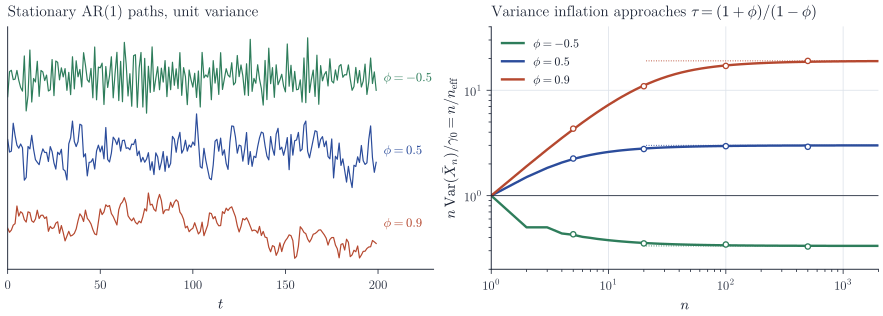
\[\frac{n}{n_{\mathrm{eff}}} = \frac{1+\phi}{1-\phi} - \frac{2\phi\,(1 - \phi^n)}{n\,(1-\phi)^2}.\]

With $\phi = 0.9$, $\tau = 19$: a run of 5,000 draws estimates the mean as precisely as 263 independent draws. With $\phi = -0.5$, $\tau = 1/3$ and the run is worth three times its length. The correction term shows that $n/n_{\mathrm{eff}}$ approaches $\tau$ at rate $1/n$, with a constant that grows like $(1-\phi)^{-2}$; for strongly correlated chains the asymptotic formula is accurate only once $n$ is a large multiple of $\tau$. Figure 1 shows this approach together with simulated values.

Sample paths of autoregressions with three coefficients, and the ratio of n to the effective sample size as a function of n — Figure 1. Left: stationary AR(1) paths with unit variance and $\phi = -0.5, 0.5, 0.9$ (offset vertically). Right: $n\,\mathrm{Var}(\bar X_n)/\gamma_0 = n/n_{\mathrm{eff}}$ from the exact formula (lines) and from 4,000 simulated runs at $n = 5, 20, 100, 500$ (circles), with the limits $\tau = (1+\phi)/(1-\phi)$ dotted.

Estimating the integrated autocorrelation time

In practice $\tau$ is unknown and must be estimated from the same run used to compute $\bar X_n$. The natural plug-in uses the sample autocovariances

\[\hat\gamma_k = \frac1n\sum_{t=1}^{n-k}(X_t - \bar X_n)(X_{t+k} - \bar X_n), \qquad \hat\rho_k = \hat\gamma_k/\hat\gamma_0 .\]

Summing over all available lags fails completely.

Proposition 2. For any data $X_1, \dots, X_n$ that are not all equal, $1 + 2\sum_{k=1}^{n-1}\hat\rho_k = 0$.

Proof. With $Y_t = X_t - \bar X_n$ and $\hat\gamma_{-k} = \hat\gamma_k$,

\[\sum_{k=-(n-1)}^{n-1}\hat\gamma_k = \frac1n\sum_{s=1}^n\sum_{t=1}^n Y_sY_t = \frac1n\Bigl(\sum_{t=1}^n Y_t\Bigr)^2 = 0,\]

since each ordered pair $(s, t)$ appears exactly once, at lag $k = t - s$. Dividing by $\hat\gamma_0 > 0$ gives the claim.

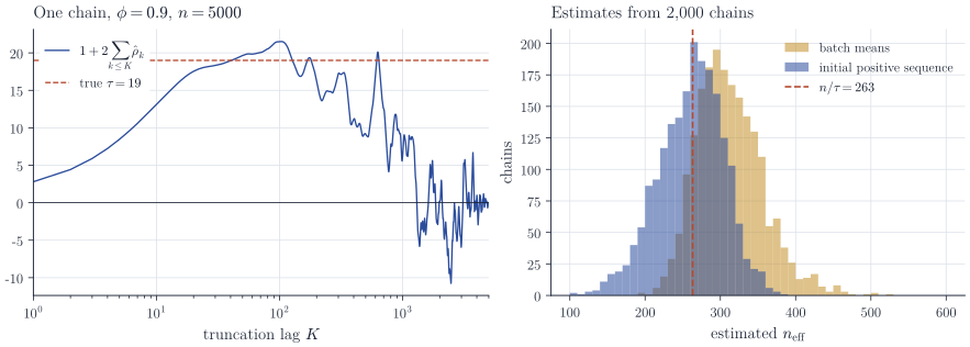
The identity reflects the fact that centring at $\bar X_n$ removes exactly the low-frequency information that $\tau$ measures. Even without centring, the full sum would be useless: each $\hat\rho_k$ has a sampling error of order $n^{-1/2}$, and the errors of $K$ lags accumulate to an error of order $\sqrt{K/n}$ or more. A consistent estimator must therefore sum only the first $K$ lags, with $K \to \infty$ (to capture all the correlation) and $K/n \to 0$ (to control the noise). The left panel of Figure 2 shows the partial sums for one chain with $\phi = 0.9$: they rise to the neighbourhood of $\tau = 19$ by lag 50 or so, then wander, and return to zero at lag $n - 1$.

Two truncation rules are widely used.

Initial sequences. For a reversible Markov chain, C. J. Geyer, “Practical Markov chain Monte Carlo” (Statistical Science, 1992), showed that the sums of adjacent pairs $\Gamma_m = \gamma_{2m} + \gamma_{2m+1}$ are positive, decreasing and convex in $m$. Since $\gamma_0\tau = \gamma_0 + 2\sum_{k\ge1}\gamma_k = -\gamma_0 + 2\sum_{m\ge0}\Gamma_m$, the initial positive sequence estimator sums the estimated $\hat\Gamma_m$ until the first one that is not positive; noise in the tail, where the true $\Gamma_m$ are tiny, is the first thing to produce a negative value. Monotone and convex versions additionally enforce the other two properties.

import numpy as np

def ess_initial_positive(x):
    """Effective sample size via Geyer's initial positive sequence."""
    n = len(x); y = x - x.mean()
    f = np.fft.rfft(y, 2 * n)
    g = np.fft.irfft(f * np.conj(f))[:n] / n   # autocovariances
    G = g[0:-1:2] + g[1::2]                    # adjacent-pair sums
    M = np.argmax(G <= 0) if np.any(G <= 0) else len(G)
    tau = (-g[0] + 2 * G[:M].sum()) / g[0]
    return n / tau

Batch means. Split the run into $b$ consecutive batches of length $m$ and compute their means $\bar Y_1, \dots, \bar Y_b$. If $m$ is large compared with $\tau$, the batch means are nearly independent with variance close to $\sigma^2_\infty/m$, so $m$ times their sample variance estimates $\sigma^2_\infty$. The rule $m \approx \sqrt n$ is common. The bias is easy to quantify with $\eqref{eq:var}$: each batch mean has variance $\gamma_0/m$ times the bracket evaluated at $m$, so the estimator targets $\gamma_0$ times that bracket rather than $\gamma_0\tau$. For the autoregression with $\phi = 0.9$, $n = 5000$ and $m = 70$, the bracket equals about $16.4$ instead of $19$, and batch means overstate the effective sample size by roughly 15%.

The right panel of Figure 2 compares the two estimators over 2,000 independent chains. Both are centred near the truth, the batch means estimator with the predicted upward bias, and both have a coefficient of variation of about 15%: an estimated effective sample size is itself a noisy quantity and should be read to one significant figure.

Partial sums of sample autocorrelations as a function of the truncation lag, and histograms of effective sample size estimates from two methods — Figure 2. AR(1) with $\phi = 0.9$ and $n = 5000$, so $\tau = 19$ and $n/\tau \approx 263$. Left: $1 + 2\sum_{k \le K}\hat\rho_k$ for one chain as a function of the truncation lag $K$ (log scale); it returns to exactly zero at $K = n - 1$. Right: estimated effective sample sizes over 2,000 chains, from the initial positive sequence and from batch means with batch length $\lfloor\sqrt n\rfloor = 70$.

Remarks

The effective sample size depends on the function being averaged: a chain may mix well for the mean of one coordinate and poorly for a tail probability or for another coordinate, and $\tau$ must be computed separately for each quantity of interest. For multivariate summaries one replaces $\sigma^2_\infty$ by the asymptotic covariance matrix of the sample mean.

Consistency of batch means and of the closely related spectral variance estimators for Markov chains is studied in J. M. Flegal and G. L. Jones, “Batch means and spectral variance estimators in Markov chain Monte Carlo” (Annals of Statistics, 2010). Current MCMC software computes effective sample sizes with variants of Geyer’s estimator that pool several chains; see A. Vehtari, A. Gelman, D. Simpson, B. Carpenter and P.-C. Bürkner, “Rank-normalization, folding, and localization: an improved $\widehat R$ for assessing convergence of MCMC” (Bayesian Analysis, 2021).