A prior on probability distributions: three constructions of the Dirichlet process

Nonparametric Bayesian inference needs priors on infinite-dimensional objects, the most basic of which is an unknown probability distribution $P$ on a sample space $\mathcal X$. Such a prior is the law of a random probability measure. Ferguson (1973, Annals of Statistics) introduced the Dirichlet process as a prior of this kind that is both rich, in that its support is large, and tractable, in that the posterior is again a Dirichlet process. It has three equivalent descriptions, and each makes a different property easy to see.

Throughout, $\mathcal X$ is a Polish space with its Borel $\sigma$-field, $G_0$ is a probability measure on $\mathcal X$ (the base measure), and $\alpha > 0$ is a constant (the concentration parameter). For $a_1, \dots, a_k \ge 0$ with positive sum, $\mathrm{Dir}(a_1, \dots, a_k)$ denotes the Dirichlet distribution on the simplex, with the convention that a coordinate with $a_j = 0$ is identically zero.

First description: Dirichlet marginals

Definition 1. A random probability measure $P$ on $\mathcal X$ is a Dirichlet process with parameters $\alpha$ and $G_0$, written $P \sim \mathrm{DP}(\alpha, G_0)$, if for every finite measurable partition $A_1, \dots, A_k$ of $\mathcal X$,

\[\bigl(P(A_1), \dots, P(A_k)\bigr) \sim \mathrm{Dir}\bigl(\alpha G_0(A_1), \dots, \alpha G_0(A_k)\bigr).\]

The definition is consistent across partitions because of the aggregation property of the Dirichlet distribution: merging two cells of a Dirichlet vector gives a Dirichlet vector whose parameter for the merged cell is the sum of the two parameters. Ferguson used this to obtain existence from Kolmogorov’s extension theorem; turning the resulting process indexed by sets into a random measure, countably additive with probability one, needs an additional argument, and the stick-breaking construction below avoids the issue entirely.

The definition gives the moments directly. For a single set $A$, the partition $\{A, A^c\}$ gives $P(A) \sim \mathrm{Beta}\bigl(\alpha G_0(A), \alpha(1 - G_0(A))\bigr)$, so

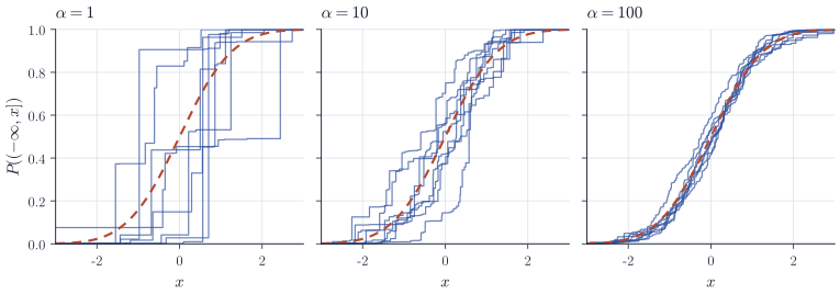
\[\E P(A) = G_0(A), \qquad \Var P(A) = \frac{G_0(A)\bigl(1 - G_0(A)\bigr)}{1 + \alpha} .\]

The base measure is the prior mean of $P$, and $\alpha$ controls how tightly $P$ concentrates around it. Figure 1 shows random distribution functions for $G_0 = N(0, 1)$: for $\alpha = 1$ they are dominated by a few large jumps, while for $\alpha = 100$ they hug the base distribution function, although they are still step functions.

Eight random distribution functions drawn from a Dirichlet process for three values of the concentration parameter, with the standard normal distribution function — Figure 1. Eight draws of the distribution function $x \mapsto P((-\infty, x])$ for $P \sim \mathrm{DP}(\alpha, N(0,1))$ with $\alpha = 1, 10, 100$ (blue), and the base distribution function $\Phi$ (dashed). Every draw is a step function; larger $\alpha$ gives more, smaller steps and less spread around $\Phi$.

The definition also yields conjugacy. Let $X_1, \dots, X_n \mid P$ be independent with distribution $P$, and $P \sim \mathrm{DP}(\alpha, G_0)$.

Theorem 2 (Ferguson). The posterior distribution of $P$ given $X_1, \dots, X_n$ is

\[\mathrm{DP}\Bigl(\alpha + n, \; \frac{\alpha G_0 + \sum_{i=1}^n \delta_{X_i}}{\alpha + n}\Bigr).\]

The heart of the proof is a finite-dimensional computation. Fix a partition $A_1, \dots, A_k$ and write $a_j = \alpha G_0(A_j)$ and $p_j = P(A_j)$. Given $p = (p_1, \dots, p_k)$, the probability that $X_1$ lands in $A_j$ is $p_j$, so the joint density of $p$ and the event $\{X_1 \in A_j\}$ is proportional to

\[p_j \prod_{l=1}^k p_l^{a_l - 1} = \prod_{l=1}^k p_l^{a_l + \mathbf 1\{l = j\} - 1},\]

and conditionally on $X_1 \in A_j$ the vector $p$ is $\mathrm{Dir}(a_1, \dots, a_j + 1, \dots, a_k)$. These are exactly the marginals of the claimed posterior, conditionally on the cell containing $X_1$. To condition on the value of $X_1$ rather than its cell, one checks that the joint law of $(X_1, P(A_1), \dots, P(A_k))$ agrees with the one implied by the claimed posterior, using partitions that refine an arbitrary set $B$ in which $X_1$ may fall; the case of $n$ observations follows by induction. Ghosal and van der Vaart, Fundamentals of Nonparametric Bayesian Inference, give a complete treatment.

The posterior mean is the convex combination

\[\E[P(A) \mid X_1, \dots, X_n] = \frac{\alpha}{\alpha + n} G_0(A) + \frac{n}{\alpha + n} \, \mathbb P_n(A),\]

where $\mathbb P_n$ is the empirical distribution. The parameter $\alpha$ acts as a prior sample size.

Second description: breaking a stick

Let $V_1, V_2, \dots$ be independent $\mathrm{Beta}(1, \alpha)$ variables and $Z_1, Z_2, \dots$ independent with distribution $G_0$, independent of the $V_k$. Define

\[w_1 = V_1, \qquad w_k = V_k \prod_{j < k}(1 - V_j) \quad (k \ge 2), \qquad P = \sum_{k=1}^\infty w_k \, \delta_{Z_k}.\]

The picture is a stick of unit length from which a $\mathrm{Beta}(1, \alpha)$ fraction is broken off at each step, the broken piece becoming the weight of a new atom placed at an independent draw from $G_0$.

Proposition 3. Almost surely $\sum_k w_k = 1$, so $P$ is a random probability measure. Moreover $\E w_k = \frac{1}{1+\alpha}\bigl(\frac{\alpha}{1+\alpha}\bigr)^{k-1}$.

Proof. By induction, $1 - \sum_{k \le K} w_k = \prod_{k \le K}(1 - V_k) =: R_K$. The sequence $R_K$ is nonnegative and nonincreasing, so it has a limit $R_\infty$, and by independence $\E R_K = \bigl(\alpha/(1+\alpha)\bigr)^K \to 0$. Monotone convergence gives $\E R_\infty = 0$, so $R_\infty = 0$ almost surely. The formula for $\E w_k$ follows from independence and $\E V_k = 1/(1+\alpha)$.

Sethuraman (1994, Statistica Sinica) showed that $P$ constructed this way is $\mathrm{DP}(\alpha, G_0)$. The key observation is a distributional fixed-point equation. Writing $P' = \sum_{k \ge 2} \bigl(w_k/(1 - V_1)\bigr)\delta_{Z_k}$, which has the same law as $P$ and is independent of $(V_1, Z_1)$,

\[P = V_1 \, \delta_{Z_1} + (1 - V_1) \, P'.\]

One checks, using standard identities for Dirichlet and beta variables, that $\mathrm{DP}(\alpha, G_0)$ satisfies the same equation in distribution, and that the equation has a unique solution among laws of random probability measures.

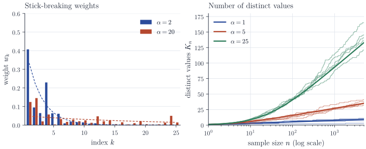
The construction makes one property obvious that the first description hides: a draw from a Dirichlet process is a discrete distribution with probability one, even when $G_0$ has a density. This is why the distribution functions in Figure 1 are step functions. The weights decay geometrically in expectation (Figure 2, left), slowly when $\alpha$ is large and quickly when it is small. Discreteness makes the Dirichlet process unsuitable as a direct prior for a density, and is the reason that it is usually used as a mixing distribution in mixture models.

Third description: a Pólya urn

Integrate $P$ out. Theorem 2 and the formula for the posterior mean give the predictive distributions of the observations:

\[\begin{equation} X_1 \sim G_0, \qquad X_{n+1} \mid X_1, \dots, X_n \sim \frac{\alpha}{\alpha + n} G_0 + \frac{1}{\alpha + n}\sum_{i=1}^n \delta_{X_i} . \label{eq:urn} \end{equation}\]

Blackwell and MacQueen (1973, Annals of Statistics) described this as a generalized Pólya urn. An urn holds balls of mass $\alpha$ spread according to $G_0$ together with one ball for each previous draw; a draw from $G_0$ produces a new value, and a draw of an old ball repeats its value. They also proved the converse: the sequence defined by $\eqref{eq:urn}$ is exchangeable, so by de Finetti’s theorem it is conditionally independent given a random probability measure, the limit of its empirical distributions, and that random measure is $\mathrm{DP}(\alpha, G_0)$.

When $G_0$ has no atoms, a draw from $G_0$ is a new value with probability one, and ties among the $X_i$ arise only from reusing old balls. The values therefore cluster. In the language of the Chinese restaurant process, observation $n + 1$ joins an existing cluster with probability proportional to its size and starts a new one with probability proportional to $\alpha$.

Proposition 4. Suppose $G_0$ has no atoms and let $K_n$ be the number of distinct values among $X_1, \dots, X_n$. Then $K_n = \sum_{i=1}^n D_i$, where the $D_i$ are independent with $D_i \sim \mathrm{Bernoulli}\bigl(\alpha/(\alpha + i - 1)\bigr)$. In particular

\[\E K_n = \sum_{i=1}^n \frac{\alpha}{\alpha + i - 1}, \qquad \Var K_n = \sum_{i=1}^n \frac{\alpha(i-1)}{(\alpha + i - 1)^2},\]

and $\E K_n / \log n \to \alpha$ as $n \to \infty$.

Proof. Let $D_i$ indicate that $X_i$ differs from $X_1, \dots, X_{i-1}$. By $\eqref{eq:urn}$ and the absence of atoms, $\P(D_i = 1 \mid X_1, \dots, X_{i-1}) = \alpha/(\alpha + i - 1)$, a constant. A sequence of indicators whose conditional success probabilities given the past are constants is independent: by induction, $\P(D_1 = d_1, \dots, D_i = d_i)$ factorizes into the product of the marginal probabilities. The moment formulas follow. Comparing the sum with $\int_0^n \alpha/(\alpha + t)\,\dd t = \alpha\log(1 + n/\alpha)$, which it exceeds by at most $1$ since the summand is decreasing, gives $\E K_n = \alpha\log n + O(1)$.

Since $\Var K_n \le \E K_n$, Chebyshev’s inequality gives $K_n/\log n \to \alpha$ in probability. The convergence also holds almost surely (Korwar and Hollander, 1973, Annals of Probability): the centred summands $D_i - \E D_i$ are independent with $\sum_{i \ge 2}\Var D_i/(\log i)^2 \le \sum_{i\ge2} \alpha/\bigl((i-1)(\log i)^2\bigr) < \infty$, so Kolmogorov’s convergence criterion and Kronecker’s lemma give $(K_n - \E K_n)/\log n \to 0$ almost surely. The number of distinct values grows without bound but only logarithmically (Figure 2, right). This is the property that makes Dirichlet process mixtures attractive: the number of clusters used to describe the data is not fixed in advance and can grow with the sample, at a rate set by $\alpha$.

Left: first twenty-five stick-breaking weights for two concentration parameters with their expectations. Right: number of distinct values against sample size for Polya urn sequences with three concentration parameters — Figure 2. Left: the first 25 stick-breaking weights of one draw for $\alpha = 2$ and $\alpha = 20$, with the expected weights $\frac{1}{1+\alpha}(\frac{\alpha}{1+\alpha})^{k-1}$ (dashed). Right: the number of distinct values $K_n$ in five Pólya urn sequences for each of $\alpha = 1, 5, 25$ (thin lines) and $\mathbb E K_n$ (thick lines), on a logarithmic $n$ axis, where $\mathbb E K_n = \alpha\log n + O(1)$ becomes close to linear with slope $\alpha$ once $n$ is large compared with $\alpha$.

Remarks

The three descriptions are used for different purposes. The marginal definition gives moments, conjugacy and posterior consistency results, and its support is easy to describe: if $G_0$ has full support, the Dirichlet process has every probability measure on $\mathcal X$ in its weak support. Stick-breaking gives simulation algorithms, truncation approximations and variational methods, and generalizes to the Pitman–Yor process, in which $V_k \sim \mathrm{Beta}(1 - d, \alpha + kd)$ and the number of distinct values grows like a power $n^d$. The urn gives collapsed Gibbs samplers for mixture models, in which $P$ is integrated out and only the partition of the data into clusters is sampled. Ghosal and van der Vaart’s book and Hjort, Holmes, Müller and Walker (eds.), Bayesian Nonparametrics, cover all three in depth.