Mixtures without a fixed number of components: Dirichlet process mixtures and collapsed Gibbs sampling

A finite mixture model asks the analyst to fix the number of components $K$ before seeing the data, and then to choose among fits with different $K$ by some criterion. A Dirichlet process mixture removes the choice from the model specification. It is a mixture with infinitely many components, of which only finitely many are ever used by a finite sample, and the number used is inferred along with everything else. The prior that the model induces on partitions of the data is what makes this work: it has a closed form, it is exchangeable, and with a conjugate base measure it leads to a Gibbs sampler that moves one observation at a time between clusters.

The model

Let $\{f(\cdot \mid \theta) : \theta \in \Theta\}$ be a family of densities on $\R^d$, the mixture kernel, and $G_0$ a probability measure on $\Theta$. A Dirichlet process mixture is the hierarchical model

\[P \sim \mathrm{DP}(\alpha, G_0), \qquad \theta_1, \dots, \theta_n \mid P \overset{\text{iid}}{\sim} P, \qquad X_i \mid \theta_i \sim f(\cdot \mid \theta_i) \text{ independently}.\]

By the stick-breaking representation $P = \sum_{k \ge 1} w_k \delta_{\phi_k}$ with $\phi_k \sim G_0$, the marginal density of each $X_i$ given $P$ is the infinite mixture $\sum_k w_k f(x \mid \phi_k)$. Because $P$ is discrete, the $\theta_i$ have ties, and observations sharing a value of $\theta$ form a cluster. It is convenient to encode this by labels $z_1, \dots, z_n$, numbered in order of first appearance, and distinct values $\phi_1, \dots, \phi_K$, so that $\theta_i = \phi_{z_i}$.

The prior on partitions

Integrating out $P$, the $\theta_i$ follow the Pólya urn: $\theta_{i}$ equals one of the earlier values with probability proportional to its multiplicity, or is a fresh draw from $G_0$ with probability proportional to $\alpha$. When $G_0$ has no atoms, fresh draws are almost surely new values, and the labels follow the Chinese restaurant process: customer $i$ joins an existing table $k$ with probability $n_k/(\alpha + i - 1)$, where $n_k$ is its current occupancy, and opens a new table with probability $\alpha/(\alpha + i - 1)$.

Multiplying these conditional probabilities along the sequence gives the probability of any labelling with $K$ clusters of sizes $n_1, \dots, n_K$. The new-table factors contribute $\alpha^K$, the factors for cluster $k$ contribute $1 \cdot 2 \cdots (n_k - 1)$ as it grows, and the denominators multiply to $\alpha(\alpha + 1)\cdots(\alpha + n - 1)$. Hence

\[\begin{equation} p(z_1, \dots, z_n) = \frac{\alpha^K \, \Gamma(\alpha)}{\Gamma(\alpha + n)} \prod_{k=1}^K (n_k - 1)! . \label{eq:eppf} \end{equation}\]

The right-hand side depends only on the cluster sizes, not on the order of the observations. The partition is therefore exchangeable, and any observation can be treated as if it were the last to arrive. This is what makes the sampler below simple.

The mixture parameters also integrate out when $G_0$ is conjugate to $f$. Given the partition, the $\phi_k$ are independent with prior $G_0$, and cluster $k$ contributes the marginal likelihood

\[m(x_{S_k}) = \int_\Theta \prod_{i \in S_k} f(x_i \mid \phi) \, G_0(\dd\phi),\]

where $S_k = \{i : z_i = k\}$. The posterior over partitions is $p(z \mid x) \propto p(z)\prod_{k} m(x_{S_k})$, a distribution on a finite but enormous set.

The collapsed Gibbs sampler

The sampler updates one label at a time from its full conditional. Fix $i$, remove observation $i$ from its cluster (deleting the cluster if it becomes empty), and let $z_{-i}$, $n_{-i,k}$ and $S_{-i,k}$ refer to the remaining $n - 1$ observations. By exchangeability of $\eqref{eq:eppf}$, the prior conditional of $z_i$ is the Chinese restaurant rule with $i$ arriving last. For the likelihood, adding $x_i$ to cluster $k$ changes the product of marginal likelihoods by the factor $m(x_{S_{-i,k}} \cup \{x_i\})/m(x_{S_{-i,k}})$, which is the posterior predictive density of $x_i$ given the other members of the cluster,

\[p(x_i \mid x_{S}) = \int_\Theta f(x_i \mid \phi) \, p(\phi \mid x_{S}) \, \dd\phi ,\]

where $p(\phi \mid x_S)$ is the posterior under prior $G_0$ given the observations in $S$; with $S = \varnothing$ this is the prior predictive. Therefore

\[\P(z_i = k \mid z_{-i}, x) \propto \begin{cases} n_{-i,k} \; p\bigl(x_i \mid x_{S_{-i,k}}\bigr), & k \text{ an existing cluster}, \\ \alpha \; p(x_i \mid \varnothing), & k \text{ a new cluster}. \end{cases}\]

This is Algorithm 3 in Neal (2000, Journal of Computational and Graphical Statistics), which also gives samplers for non-conjugate base measures. Each update needs the counts and sufficient statistics of the current clusters, which are updated in constant time when an observation moves.

For the example we use bivariate normal clusters with known covariance $\sigma^2 I$ and base measure $G_0 = N(\mu_0, \tau_0^2 I)$ for the cluster means. For a cluster $S$ with $m$ members and sum $\Sigma_S = \sum_{j \in S} x_j$, standard normal conjugacy gives the posterior $\phi \mid x_S \sim N(\mu_S, s_S^2 I)$ with

\[s_S^2 = \Bigl(\frac{1}{\tau_0^2} + \frac{m}{\sigma^2}\Bigr)^{-1}, \qquad \mu_S = s_S^2\Bigl(\frac{\mu_0}{\tau_0^2} + \frac{\Sigma_S}{\sigma^2}\Bigr),\]

and the predictive density is $N\bigl(x_i; \mu_S, (\sigma^2 + s_S^2) I\bigr)$. One sweep of the sampler is then short:

def sweep(X, z, cnt, sm, alpha, rng):
    empty = (np.zeros(1), np.zeros((1, 2)))
    for i in rng.permutation(len(X)):
        k = z[i]; cnt[k] -= 1; sm[k] = sm[k] - X[i]
        if cnt[k] == 0:              # drop the emptied cluster
            cnt.pop(k); sm.pop(k); z[z > k] -= 1
        c, s = np.array(cnt, float), np.array(sm)
        old = np.log(c) + log_pred(X[i], c, s)
        new = np.log(alpha) + log_pred(X[i], *empty)
        logw = np.append(old, new)
        w = np.exp(logw - logw.max())
        k = rng.choice(len(w), p=w / w.sum())
        if k == len(cnt):            # open a new cluster
            cnt.append(0); sm.append(np.zeros(2))
        z[i] = k; cnt[k] += 1; sm[k] = sm[k] + X[i]

Here log_pred evaluates the log predictive density above for every cluster at once from the counts cnt and coordinate sums sm.

An example

We simulate $n = 300$ points from four bivariate normal components with standard deviation $0.5$ and mixing proportions $0.35, 0.30, 0.20, 0.15$, and fit the model with $\sigma = 0.5$, $\tau_0 = 3$, $\mu_0$ equal to the sample mean (a mild empirical Bayes choice) and $\alpha = 1$. The sampler starts with all points in one cluster and runs for 400 sweeps.

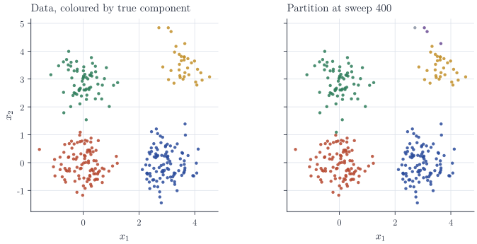
Left: simulated two-dimensional data coloured by true component. Right: the partition at the final sweep of the Gibbs sampler, which recovers the four groups and adds a few tiny clusters — Figure 1. Left: 300 points from a four-component normal mixture, coloured by component. Right: the partition at the last of 400 sweeps of the collapsed Gibbs sampler (colours are assigned by cluster size and carry no other meaning). The four groups are recovered, together with two very small clusters of outlying points.

The four groups are found within the first few dozen sweeps, after which the sampler mostly moves a handful of outlying points between the large clusters and small clusters of their own (Figure 1). Label switching, the usual nuisance in sampling finite mixtures, does not arise: the state is a partition, and the cluster numbering carries no information.

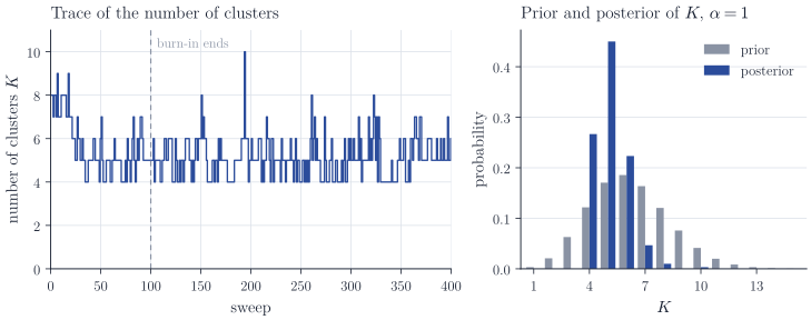
Left: trace plot of the number of clusters over 400 sweeps. Right: prior and posterior probabilities of the number of clusters — Figure 2. Left: number of clusters $K$ at each sweep; the dashed line marks the end of the 100 discarded sweeps. Right: prior distribution of $K$ for $n = 300$ and $\alpha = 1$ (grey), computed exactly from the representation of $K_n$ as a sum of independent Bernoulli$(\alpha/(\alpha + i - 1))$ variables, and the posterior frequencies of $K$ over sweeps 101 to 400 (blue).

Figure 2 summarizes the number of clusters. The prior, by the Chinese restaurant process, puts $K$ near $\sum_{i \le 300} 1/i \approx 6.3$ with considerable spread. In this run the posterior concentrates on 4 to 6 clusters, with estimated probabilities of about $0.27$, $0.45$ and $0.22$, and puts its mode at 5 rather than at the true value 4 (with another data set or seed the mode may well be 4; the spread over 5 and 6 is the stable feature). The extra clusters are the small groups of outlying points visible in Figure 1.

What the posterior on $K$ means

It is tempting to read the posterior of $K$ as inference about the number of components in the population. This is not justified. Miller and Harrison (2014, Journal of Machine Learning Research) proved that when data come from a finite mixture of components in the kernel family, the posterior probability that a Dirichlet process mixture has exactly the true number of clusters does not tend to one as $n \to \infty$; under broad conditions it stays bounded away from one. The reason is visible in $\eqref{eq:eppf}$. Moving one observation out of a cluster of size $n_k$ into a new singleton multiplies the prior probability of the partition by $\alpha/(n_k - 1)$, which is of order $1/n$; but there are of order $n$ observations that could be split off, and a point in the tail of a component is fitted about as well by its own cluster as by the component’s. Collectively, partitions with one extra tiny cluster therefore keep posterior probability that does not vanish. The density estimate is unaffected, since tiny clusters carry negligible weight, and Dirichlet process mixtures do give consistent density estimates under mild conditions. When the number of components is itself the object of inference, a mixture of finite mixtures, with an explicit prior on $K$, is the appropriate model; Miller and Harrison (2018, Journal of the American Statistical Association) show that it can be sampled with the same kind of algorithm.

Remarks

The concentration parameter $\alpha$ governs the prior number of clusters, $\E K_n \approx \alpha\log n$, and can be given its own prior and updated within the sampler; Escobar and West (1995, Journal of the American Statistical Association) give a convenient auxiliary-variable update for a gamma prior on $\alpha$. With unknown cluster covariances, a normal–inverse-Wishart base measure keeps the model conjugate, and the predictive density becomes a multivariate $t$. Single-site Gibbs updates can be slow to merge or split large clusters, because moving one point at a time through a low-probability intermediate state is required; split–merge Metropolis–Hastings moves (Jain and Neal, 2004, Journal of Computational and Graphical Statistics) address this.

The model

The prior on partitions

The collapsed Gibbs sampler

An example

What the posterior on \(K\) means

Remarks