Minimizing an empirical criterion: M-estimators and the sandwich variance

The sample mean minimizes $\sum_i (X_i - \theta)^2$, the sample median minimizes $\sum_i \abs{X_i - \theta}$, and the maximum likelihood estimator minimizes $-\sum_i \log p_\theta(X_i)$. Each is the minimizer of an empirical average of a loss, and each estimates the minimizer of the corresponding expected loss. Huber (“Robust estimation of a location parameter”, Annals of Mathematical Statistics, 1964) called such estimators M-estimators, for estimators of maximum likelihood type. Treating them together has two advantages. The asymptotic theory is proved once, and the target of estimation is defined by the loss itself, so the theory does not require a correctly specified model.

Setting

Let $X_1, \dots, X_n$ be i.i.d. with law $P$ on a measurable space $\mathcal X$, and let $\Theta \subseteq \R^p$. A loss $\rho : \mathcal X \times \Theta \to \R$ is given, measurable in $x$ for each $\theta$, with $\E \abs{\rho(X, \theta)} < \infty$ for every $\theta$. Put

\[M_n(\theta) = \frac1n \sum_{i=1}^n \rho(X_i, \theta), \qquad M(\theta) = \E\, \rho(X, \theta).\]

The target is $\theta_0 = \argmin_\theta M(\theta)$, assumed to exist, and an M-estimator is any $\hat\theta_n$ that minimizes $M_n$, possibly up to a small error. When $\rho$ is differentiable in $\theta$ one usually solves the first-order condition instead. More generally, given a vector-valued $\psi : \mathcal X \times \Theta \to \R^p$ with $\E \lVert \psi(X, \theta) \rVert < \infty$, a Z-estimator solves

\[\Psi_n(\theta) = \frac1n \sum_{i=1}^n \psi(X_i, \theta) = 0, \qquad \text{targeting the root } \theta_0 \text{ of } \Psi(\theta) = \E\, \psi(X, \theta).\]

Some familiar cases, in a location model with residual $u = x - \theta$ and estimating equation $\sum_i \varphi(X_i - \theta) = 0$:

$\rho(u) = u^2/2$ and $\varphi(u) = u$ give the sample mean; the target is $\E X$.
$\rho(u) = \abs{u}$ and $\varphi(u) = \sign(u)$ give the sample median; the target is any median of $P$.
Huber’s loss $\rho_k(u) = u^2/2$ for $\abs{u} \le k$ and $k \abs{u} - k^2/2$ otherwise has $\varphi_k(u) = \max(-k, \min(k, u))$. It behaves like the mean for small residuals and like the median for large ones.
In regression with covariates $z$, $\rho(x, \theta) = \tau u - u \mathbf 1\{u < 0\}$ with $u = y - z^\top \theta$ gives the $\tau$-th regression quantile.

The equation $\Psi(\theta_0) = 0$ is what pins down the target. For the mean and median it reproduces the usual population quantities. For maximum likelihood under a misspecified model it defines the parameter closest to $P$ in Kullback–Leibler divergence, which is the reason the theory below is stated in terms of $P$ and never in terms of a model.

Consistency

Consistency rests on two requirements: the empirical criterion must approximate the population criterion uniformly, and the population minimum must be well separated, so that parameters far from $\theta_0$ cannot come close to the minimal value.

Theorem 1. Let $d$ be a metric on $\Theta$. Suppose that

$\sup_{\theta \in \Theta} \abs{M_n(\theta) - M(\theta)} \xrightarrow{p} 0$;
for every $\varepsilon > 0$, $\inf\{M(\theta) : d(\theta, \theta_0) \ge \varepsilon\} > M(\theta_0)$;
$M_n(\hat\theta_n) \le M_n(\theta_0) + o_P(1)$.

Then $\hat\theta_n \xrightarrow{p} \theta_0$.

Proof. Write $\Delta_n = \sup_\theta \abs{M_n(\theta) - M(\theta)}$. By condition 3 and two applications of the definition of $\Delta_n$,

\[M(\hat\theta_n) - M(\theta_0) \le \bigl(M(\hat\theta_n) - M_n(\hat\theta_n)\bigr) + \bigl(M_n(\theta_0) - M(\theta_0)\bigr) + o_P(1) \le 2\Delta_n + o_P(1),\]

so $M(\hat\theta_n) - M(\theta_0) \xrightarrow{p} 0$. Given $\varepsilon > 0$, condition 2 provides $\eta > 0$ such that $d(\theta, \theta_0) \ge \varepsilon$ implies $M(\theta) \ge M(\theta_0) + \eta$. Hence $\P(d(\hat\theta_n, \theta_0) \ge \varepsilon) \le \P(M(\hat\theta_n) - M(\theta_0) \ge \eta) \to 0$.

(If $\hat\theta_n$ is not measurable the probabilities are outer probabilities; nothing else changes.) Condition 2 is stronger than uniqueness of the minimizer. When $\Theta$ is compact and $M$ is continuous, uniqueness implies it, because a continuous function attains its infimum on the compact set $\{d(\theta, \theta_0) \ge \varepsilon\}$. Condition 1 is a uniform law of large numbers. It holds, for example, when $\Theta$ is compact, $\theta \mapsto \rho(x, \theta)$ is continuous for every $x$, and $\sup_\theta \abs{\rho(x, \theta)} \le m(x)$ with $\E\, m(X) < \infty$. For losses convex in $\theta$, such as all four examples above, compactness can be dropped. Pointwise convergence of convex functions on an open convex set is automatically uniform on compact subsets (the version for convergence in probability follows by passing to almost surely convergent subsequences along a countable dense set), and convexity confines the minimizer of $M_n$ to a neighbourhood of $\theta_0$ once $M_n$ exceeds $M_n(\theta_0)$ on the boundary of that neighbourhood.

Asymptotic normality

For the limiting distribution it is convenient to work with the estimating equation. The idea is a one-term expansion: $0 \approx \Psi_n(\hat\theta_n) \approx \Psi_n(\theta_0) + \dot\Psi_n(\theta_0)(\hat\theta_n - \theta_0)$, where $\dot\Psi_n$ is the $p \times p$ Jacobian. The central limit theorem applies to $\Psi_n(\theta_0)$, which is an average of mean-zero vectors, and the law of large numbers applies to the Jacobian. The work lies in controlling the Jacobian at points between $\theta_0$ and $\hat\theta_n$, and this is what the local domination condition below is for. Write $\dot\psi(x, \theta) = \partial \psi(x, \theta) / \partial \theta^\top$.

Theorem 2. Assume that $\theta_0$ is an interior point of $\Theta$ with $\Psi(\theta_0) = 0$, and that

$\hat\theta_n \xrightarrow{p} \theta_0$ and $\Psi_n(\hat\theta_n) = o_P(n^{-1/2})$;
$B = \E\, \psi(X, \theta_0) \psi(X, \theta_0)^\top$ is finite;
there is a closed ball $U$ around $\theta_0$ such that for every $x$ the map $\theta \mapsto \psi(x, \theta)$ is continuously differentiable on $U$, and $\sup_{\theta \in U} \lVert \dot\psi(x, \theta) \rVert \le m(x)$ with $\E\, m(X) < \infty$;
$V = \E\, \dot\psi(X, \theta_0)$ is nonsingular.

Then

\[\sqrt n (\hat\theta_n - \theta_0) = -V^{-1} \frac{1}{\sqrt n} \sum_{i=1}^n \psi(X_i, \theta_0) + o_P(1) \rightsquigarrow N_p\bigl(0, \; V^{-1} B V^{-\top}\bigr).\]

Proof. On the event $\{\hat\theta_n \in U\}$, whose probability tends to one, the segment from $\theta_0$ to $\hat\theta_n$ lies in $U$ by convexity of the ball. The fundamental theorem of calculus, applied for each fixed $x$ to $t \mapsto \psi(x, \theta_0 + t(\hat\theta_n - \theta_0))$, gives after averaging

\[\Psi_n(\hat\theta_n) - \Psi_n(\theta_0) = A_n (\hat\theta_n - \theta_0), \qquad A_n = \frac1n \sum_{i=1}^n \int_0^1 \dot\psi\bigl(X_i, \theta_0 + t(\hat\theta_n - \theta_0)\bigr) \, \dd t .\]

We show $A_n \xrightarrow{p} V$. For $\delta > 0$ small enough that the closed $\delta$-ball around $\theta_0$ lies in $U$, let

\[w_\delta(x) = \sup_{\lVert \theta - \theta_0 \rVert \le \delta} \bigl\lVert \dot\psi(x, \theta) - \dot\psi(x, \theta_0) \bigr\rVert .\]

By continuity in $\theta$ the supremum may be taken over a countable dense set, so $w_\delta$ is measurable. It satisfies $w_\delta \le 2m$ and $w_\delta(x) \to 0$ as $\delta \downarrow 0$ for every $x$, so $\E\, w_\delta(X) \to 0$ by dominated convergence with dominating function $2m$. Fix $\eta > 0$ and choose $\delta$ with $\E\, w_\delta(X) < \eta$. On $\{\lVert \hat\theta_n - \theta_0 \rVert \le \delta\}$,

\[\Bigl\lVert A_n - \frac1n \sum_{i=1}^n \dot\psi(X_i, \theta_0) \Bigr\rVert \le \frac1n \sum_{i=1}^n w_\delta(X_i),\]

and the right-hand side converges almost surely to $\E\, w_\delta(X) < \eta$ by the strong law. Since also $n^{-1} \sum_i \dot\psi(X_i, \theta_0) \to V$ almost surely, $\P(\lVert A_n - V \rVert > 2\eta) \to 0$. As $\eta$ was arbitrary, $A_n \xrightarrow{p} V$; because $V$ is nonsingular and inversion is continuous there, $A_n$ is invertible with probability tending to one and $A_n^{-1} \xrightarrow{p} V^{-1}$.

On the event where $\hat\theta_n \in U$ and $A_n$ is invertible,

\[\sqrt n (\hat\theta_n - \theta_0) = A_n^{-1} \bigl( \sqrt n\, \Psi_n(\hat\theta_n) - \sqrt n\, \Psi_n(\theta_0) \bigr) = -A_n^{-1} \sqrt n\, \Psi_n(\theta_0) + o_P(1).\]

The vectors $\psi(X_i, \theta_0)$ are i.i.d. with mean $\Psi(\theta_0) = 0$ and covariance $B$, so $\sqrt n\, \Psi_n(\theta_0) \rightsquigarrow N_p(0, B)$ and in particular $\sqrt n\, \Psi_n(\theta_0) = O_P(1)$. Replacing $A_n^{-1}$ by $V^{-1}$ therefore costs $o_P(1)$, and Slutsky’s lemma gives the limit law $N_p(0, V^{-1} B V^{-\top})$.

The representation in the display is often more useful than the limit law. It says that $\hat\theta_n$ is asymptotically linear with influence function $-V^{-1} \psi(x, \theta_0)$, so the joint behaviour of several M-estimators, or of an M-estimator and another average, follows from the multivariate central limit theorem.

The sandwich

The covariance $V^{-1} B V^{-\top}$ has two ingredients. The “bread” $V$ is the curvature of the population criterion at $\theta_0$; the “meat” $B$ is the variance of the estimating function. A flatter criterion makes the minimizer harder to locate, and a noisier estimating function moves the empirical root further from $\theta_0$.

For maximum likelihood, $\psi(x, \theta) = -\nabla_\theta \log p_\theta(x)$. If the model is correct, $P = P_{\theta_0}$, and differentiation under the integral sign is permitted twice (for instance under a local domination condition of the type in Theorem 2 applied to the first two derivatives of $p_\theta$), then both $B$ and $V$ equal the Fisher information $I(\theta_0)$ and the sandwich collapses to $I(\theta_0)^{-1}$. The identity $B = V$ is a property of the model, and it is the first casualty of misspecification. The sandwich itself remains valid whenever the conditions of Theorem 2 hold.

Both ingredients have plug-in estimators,

\[\hat V_n = \frac1n \sum_{i=1}^n \dot\psi(X_i, \hat\theta_n), \qquad \hat B_n = \frac1n \sum_{i=1}^n \psi(X_i, \hat\theta_n) \psi(X_i, \hat\theta_n)^\top .\]

The argument used for $A_n$ in the proof shows $\hat V_n \xrightarrow{p} V$ under the conditions of Theorem 2. Consistency of $\hat B_n$ follows in the same way if $\theta \mapsto \psi(x, \theta)\psi(x, \theta)^\top$ is continuous on $U$ and dominated there by an integrable function. Standard errors from $\hat V_n^{-1} \hat B_n \hat V_n^{-\top} / n$ are the heteroskedasticity-robust standard errors of regression and the robust standard errors of generalized estimating equations.

Huber’s estimator

In the location problem with $P$ symmetric about $\theta_0$, having a density $f$ that is continuous and positive at $\theta_0$ and no atoms at $\theta_0 \pm k$, take $\psi(x, \theta) = \varphi_k(x - \theta)$. Symmetry and oddness of $\varphi_k$ give $\Psi(\theta_0) = 0$, and $\theta_0$ is the only root because $\Psi$ is nonincreasing and, by the density assumption, strictly decreasing near $\theta_0$. The Huber score is not differentiable at $\pm k$, so condition 3 of Theorem 2 fails as stated. The population map is nevertheless differentiable: since $\varphi_k$ is 1-Lipschitz with derivative $\mathbf 1\{\abs{u} < k\}$ off the two points $\pm k$, which carry no mass under the law of $X - \theta_0$, dominated convergence (difference quotients bounded by 1) gives $\Psi'(\theta_0) = -\P(\abs{X - \theta_0} < k)$. The conclusion of Theorem 2 survives with this $V$; the extension from pointwise differentiability of $\psi$ to differentiability of $\Psi$ plus a Lipschitz condition in $\theta$ is treated in Chapter 5 of van der Vaart, Asymptotic Statistics. Writing $\varepsilon = X - \theta_0$, the asymptotic variance is

\[\sigma^2(k) = \frac{B}{V^2} = \frac{\E \min(\varepsilon^2, k^2)}{\P(\abs{\varepsilon} < k)^2}.\]

As $k \to \infty$ this tends to $\Var(\varepsilon)$, the variance of the mean, provided it is finite. As $k \downarrow 0$ the numerator is $k^2 (1 + o(1))$ and the denominator is $(2k f(\theta_0))^2 (1 + o(1))$, which recovers the median’s asymptotic variance $1/(4 f(\theta_0)^2)$.

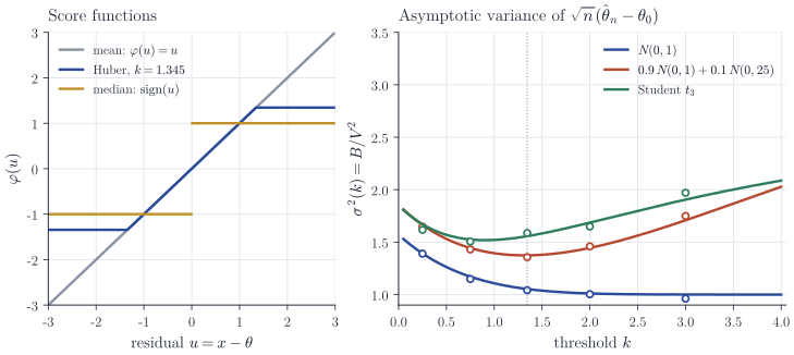
Left: score functions of the mean, the Huber estimator and the median. Right: asymptotic variance of the Huber estimator as a function of the threshold for three error laws, with Monte Carlo points. — Figure 1. Left: the estimating functions $\varphi$ of the mean, the median and Huber's estimator. Right: $\sigma^2(k)$ computed by numerical integration for three symmetric error laws (curves), and $n$ times the Monte Carlo variance of the Huber estimator with $n = 200$ and $4000$ replications (circles). The dotted line marks $k = 1.345$. The variances of the mean are $1$, $3.4$ and $3$, respectively.

The figure shows the trade-off that motivates the estimator. Under normal errors the mean is optimal and $k = 1.345$ costs about five percent in variance. Under a ten percent contamination by a normal with five times the scale, or under $t_3$ errors, the mean’s variance is $3.4$ or $3$, while Huber’s estimator with the same $k$ attains $1.37$ and $1.56$. In both heavy-tailed cases the curve has an interior minimum, so neither the mean nor the median is the best member of the family. The Monte Carlo points agree with the curves to within simulation error at $n = 200$.

Remarks

In practice the scale of $\varepsilon$ is unknown and $k$ is applied to standardized residuals $(X_i - \theta)/\hat s$ with a robust scale estimate $\hat s$. When $P$ is symmetric and $\hat s$ converges in probability to some $s > 0$, the derivative of the location equation with respect to the scale vanishes at $(\theta_0, s)$ by symmetry, the two equations decouple asymptotically, and the asymptotic variance of $\sqrt n(\hat\theta_n - \theta_0)$ is $s^2$ times the formula above evaluated for $\varepsilon / s$; without symmetry the joint sandwich for location and scale is needed.

Theorem 2 requires the estimating function to be smooth in $\theta$ for every observation. The median and quantile regression violate this, and their asymptotic normality is obtained from smoothness of $\Psi$ alone together with empirical process bounds, or for convex criteria from a direct convexity argument. Huber’s Robust Statistics and Chapter 5 of van der Vaart’s Asymptotic Statistics treat both routes.