LU, Cholesky, QR and the SVD: what each factorization buys

Almost every numerical computation in statistics with a dense matrix passes through one of four factorizations. Each writes a matrix as a product of factors that are cheap to work with: triangular matrices, which are inverted by substitution in $O(n^2)$ operations; orthogonal matrices, whose inverse is the transpose and which do not amplify rounding errors; and diagonal matrices. The factorizations differ in which matrices they apply to, what they cost, and how much they reveal. Below, each factorization comes with a proof of existence and uniqueness, followed by the comparison that matters most in statistical practice: how to solve least-squares problems.

Flop counts below are leading-order counts of floating-point operations for dense $n \times n$ matrices, or $n \times p$ matrices with $n \ge p$, as in Golub and Van Loan, Matrix Computations.

LU: Gaussian elimination written as a product

Gaussian elimination subtracts multiples of row $k$ from the rows below it to create zeros under the diagonal in column $k$. Each step is multiplication on the left by a unit lower-triangular matrix, and the product of their inverses is again unit lower triangular. What remains is upper triangular, so elimination computes $A = LU$.

Theorem 1 (LU factorization). Let $A \in \R^{n \times n}$ and let $A_k$ be its leading $k \times k$ submatrix. There exist a unit lower-triangular $L$ and a nonsingular upper-triangular $U$ with $A = LU$ if and only if $\det A_k \neq 0$ for $k = 1, \dots, n$. The factorization is then unique.

Proof. If $A = LU$, then $A_k = L_k U_k$ for the leading blocks, because the factors are triangular, so $\det A_k = \prod_{i \le k} u_{ii} \neq 0$.

Conversely, argue by induction on $n$; the case $n = 1$ is trivial. Partition

\[A = \begin{pmatrix} A_{n-1} & b \\ c^\top & a \end{pmatrix}\]

and let $A_{n-1} = L'U'$ by the induction hypothesis. Put

\[L = \begin{pmatrix} L' & 0 \\ c^\top U'^{-1} & 1 \end{pmatrix}, \qquad U = \begin{pmatrix} U' & L'^{-1} b \\ 0 & a - c^\top A_{n-1}^{-1} b \end{pmatrix}.\]

Multiplying the blocks gives $LU = A$; the bottom-right entry is $c^\top U'^{-1}L'^{-1} b + a - c^\top A_{n-1}^{-1} b = a$. The last pivot $a - c^\top A_{n-1}^{-1} b$ equals $\det A / \det A_{n-1}$, by the block determinant formula, and is nonzero.

For uniqueness, $L_1 U_1 = L_2 U_2$ gives $L_2^{-1} L_1 = U_2 U_1^{-1}$. The left side is unit lower triangular and the right side is upper triangular, so both equal $I$.

The condition on leading minors fails for perfectly good matrices, such as $\bigl(\begin{smallmatrix} 0 & 1 \\ 1 & 0 \end{smallmatrix}\bigr)$, and near-failures are numerically harmful. For $A = \bigl(\begin{smallmatrix} \delta & 1 \\ 1 & 1 \end{smallmatrix}\bigr)$ with small $\delta > 0$, elimination gives $l_{21} = 1/\delta$ and $u_{22} = 1 - 1/\delta$. When $\delta$ is much smaller than the unit roundoff (say $\delta = 10^{-20}$ in double precision), $u_{22}$ is stored as $-1/\delta$, and the computed product $LU$ has $(2,2)$ entry $0$ instead of $1$: the information in $a_{22}$ is lost. Partial pivoting swaps rows so that the pivot is the largest entry in absolute value in its column, which keeps all multipliers in $[-1, 1]$. Every nonsingular $A$ then has a factorization $PA = LU$ with $P$ a permutation matrix.

LU costs $\tfrac23 n^3$ flops. Once it is available, each system $Ax = b$ costs two triangular solves, $O(n^2)$, and $\det A = \pm\prod_i u_{ii}$, with the sign given by the parity of $P$. Forming $A^{-1}$ explicitly is rarely needed: $A^{-1}B$ is computed by solving with the factors.

Cholesky: LU for positive definite matrices

For symmetric positive definite matrices elimination needs no pivoting, and symmetry halves the work.

Theorem 2 (Cholesky factorization). A symmetric matrix $A \in \R^{n \times n}$ is positive definite if and only if $A = LL^\top$ for some lower-triangular $L$ with positive diagonal entries. Such an $L$ is unique.

Proof. If $A = LL^\top$ with $L$ nonsingular, then $x^\top A x = \lVert L^\top x\rVert^2 > 0$ for $x \neq 0$.

For the converse, induct on $n$. Partition $A = \bigl(\begin{smallmatrix} a & b^\top \\ b & C \end{smallmatrix}\bigr)$ with $a = e_1^\top A e_1 > 0$. The Schur complement $S = C - bb^\top/a$ is positive definite: for $x \in \R^{n-1}$, $x \neq 0$, the vector $z = (-b^\top x/a,\, x)$ is nonzero and

\[0 < z^\top A z = \frac{(b^\top x)^2}{a} - \frac{2 (b^\top x)^2}{a} + x^\top C x = x^\top S x .\]

By induction $S = L_1 L_1^\top$, and

\[L = \begin{pmatrix} \sqrt a & 0 \\ b/\sqrt a & L_1 \end{pmatrix} \quad\text{satisfies}\quad LL^\top = \begin{pmatrix} a & b^\top \\ b & bb^\top/a + L_1 L_1^\top \end{pmatrix} = A .\]

For uniqueness, $L_1L_1^\top = L_2 L_2^\top$ gives $L_2^{-1}L_1 = L_2^\top L_1^{-\top}$, which is both lower and upper triangular, hence a diagonal matrix $\Delta$ with positive entries. Then $\Delta = \Delta^{-\top} = \Delta^{-1}$, so $\Delta^2 = I$ and $\Delta = I$.

The proof is an algorithm: compute the first column of $L$, form the Schur complement, repeat. It costs $\tfrac13 n^3$ flops, and in exact arithmetic it fails, by meeting a nonpositive pivot, exactly when $A$ is not positive definite, which makes it the standard numerical test of positive definiteness. For a covariance matrix $\Sigma = LL^\top$, the Gaussian log-density needs $\log\det\Sigma = 2\sum_i \log l_{ii}$ and $(x-\mu)^\top\Sigma^{-1}(x-\mu) = \lVert L^{-1}(x-\mu)\rVert^2$, the latter by one forward substitution; and $\mu + LZ$ with $Z \sim N(0, I_n)$ has law $N(\mu, \Sigma)$.

QR: orthogonalizing the columns

Let $A \in \R^{n \times p}$ have full column rank $p$.

Theorem 3 (QR factorization). There is a unique pair $Q \in \R^{n \times p}$ with orthonormal columns and $R \in \R^{p \times p}$ upper triangular with positive diagonal such that $A = QR$. Moreover, $R^\top$ is the Cholesky factor of $A^\top A$.

Proof. The matrix $A^\top A$ is positive definite because $A$ has full column rank. By Theorem 2, $A^\top A = R^\top R$ with $R$ upper triangular with positive diagonal. Set $Q = AR^{-1}$; then $Q^\top Q = R^{-\top} A^\top A R^{-1} = I_p$. If $A = QR$ is any factorization of the stated form, then $A^\top A = R^\top Q^\top Q R = R^\top R$, and uniqueness in Theorem 2 determines $R$, hence $Q = AR^{-1}$.

The proof is a poor algorithm, for reasons that the next section makes precise. Gram–Schmidt orthogonalization of the columns of $A$ also produces $Q$ and $R$, but in floating point the computed columns of $Q$ can lose orthogonality badly. The standard method applies Householder reflections $H = I - 2vv^\top/(v^\top v)$ from the left: the first maps column one of $A$ onto a multiple of $e_1$, the second acts on rows $2, \dots, n$ of what remains, and so on, until $H_p\cdots H_1 A$ is upper triangular. Each $H_k$ is orthogonal and symmetric, so $Q$ is the first $p$ columns of $H_1 \cdots H_p$. Orthogonal transformations preserve Euclidean norms, so rounding errors committed at one step are not magnified at later steps. The cost is $2np^2 - \tfrac23 p^3$ flops.

QR is the natural tool for least squares. Complete $Q$ to an orthogonal matrix $(Q, Q_\perp) \in \R^{n \times n}$. For every $\beta$,

\[\lVert y - A\beta\rVert^2 = \lVert Q^\top y - R\beta\rVert^2 + \lVert Q_\perp^\top y\rVert^2 ,\]

since $Q^\top A = R$ and $Q_\perp^\top A = 0$. The second term does not depend on $\beta$, and the first vanishes at the solution of the triangular system $R\hat\beta = Q^\top y$. The residual norm is $\lVert Q_\perp^\top y\rVert$, and $A^\top A$ is never formed.

The SVD: everything, at a price

Theorem 4 (Singular value decomposition). Every $A \in \R^{n \times p}$ can be written $A = U\Sigma V^\top$ with $U \in \R^{n \times n}$ and $V \in \R^{p \times p}$ orthogonal and $\Sigma \in \R^{n \times p}$ zero except for diagonal entries $\sigma_1 \ge \sigma_2 \ge \cdots \ge 0$.

Proof. By the spectral theorem, $A^\top A = V\Lambda V^\top$ with $V$ orthogonal and $\lambda_1 \ge \cdots \ge \lambda_p \ge 0$; the eigenvalues are nonnegative because $\lambda_j = \lVert Av_j\rVert^2$. Let $r$ be the number of positive $\lambda_j$, put $\sigma_j = \sqrt{\lambda_j}$ and $u_j = Av_j/\sigma_j$ for $j \le r$. These vectors are orthonormal, because $u_i^\top u_j = v_i^\top A^\top A v_j/(\sigma_i\sigma_j) = \lambda_j \delta_{ij}/(\sigma_i\sigma_j) = \delta_{ij}$. Extend them to an orthonormal basis $u_1, \dots, u_n$ of $\R^n$. Then $Av_j = \sigma_j u_j$ for $j \le r$ and $Av_j = 0$ for $j > r$, since $\lVert Av_j\rVert^2 = \lambda_j = 0$. In matrix form $AV = U\Sigma$.

The SVD reveals the rank (the number of nonzero $\sigma_j$, and numerically the number above a tolerance), gives the pseudoinverse $A^+ = \sum_{j \le r} \sigma_j^{-1} v_j u_j^\top$ and, for $n \ge p$ and full column rank, the 2-norm condition number $\kappa_2(A) = \sigma_1/\sigma_p$, and by the Eckart–Young theorem its truncation $\sum_{j \le k}\sigma_j u_j v_j^\top$ is a best rank-$k$ approximation of $A$ in both the spectral and the Frobenius norm. For symmetric positive semi-definite matrices it coincides with the eigendecomposition. The proof above is again not how the SVD is computed: production algorithms first reduce $A$ to bidiagonal form with Householder reflections and then iterate, at a cost that is a modest multiple of QR’s. One pays for the SVD when the rank is in doubt or when the singular values themselves are wanted.

Least squares: normal equations or QR?

The normal equations $A^\top A \beta = A^\top y$ can be solved by Cholesky at a cost of about $np^2 + \tfrac13 p^3$ flops, roughly half the cost of Householder QR when $n \gg p$. The catch is conditioning. Since $A^\top A = V\Sigma^\top\Sigma V^\top$,

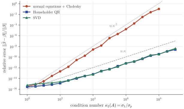
\[\kappa_2(A^\top A) = \frac{\sigma_1^2}{\sigma_p^2} = \kappa_2(A)^2 .\]

Forming $A^\top A$ in floating point with unit roundoff $u$ (about $1.1 \times 10^{-16}$ in double precision) commits relative errors of order $u$ in its entries, and a linear system with condition number $\kappa^2$ turns those into relative errors of order $u\kappa^2$ in the solution. Householder QR, in contrast, is backward stable: the computed $\hat\beta$ is the exact least-squares solution for a matrix $A + \delta A$ and response $y + \delta y$ with $\lVert\delta A\rVert \le c\, u \lVert A\rVert$ and $\lVert\delta y\rVert \le c\, u\lVert y\rVert$, where $c$ depends only on the dimensions. When the residual is small, the sensitivity of the least-squares solution to such perturbations is proportional to $\kappa_2(A)$, so QR achieves accuracy of order $u\kappa$.

Figure 1 shows the effect on simulated problems with prescribed condition numbers and zero residual. The normal equations lose twice as many digits as QR, and for $\kappa_2(A)$ above about $10^8$ the computed $A^\top A$ is no longer numerically positive definite and the Cholesky step fails. QR and the SVD are indistinguishable.

Relative error of least-squares solutions against condition number for normal equations, QR and SVD — Figure 1. Median relative error over 20 random problems with $n = 100$, $p = 10$, $A = U\,\mathrm{diag}(\sigma_j)\,V^\top$ with log-spaced singular values from $1$ to $1/\kappa$, and $y = A\beta$ exactly. Dashed and dotted lines are $u\kappa$ and $u\kappa^2$. The normal-equation curve stops at the first $\kappa$ for which the Cholesky factorization of the computed $A^\top A$ failed in at least one of the 20 problems.

When the residual $r = y - A\hat\beta$ is large, the least-squares problem is itself sensitive at order $\kappa^2$: first-order perturbation bounds contain a term proportional to $\kappa_2(A)^2\,\lVert r\rVert / (\lVert A\rVert\,\lVert\hat\beta\rVert)$, which no algorithm can avoid. The advantage of QR is therefore largest for nearly consistent systems, but it is never a disadvantage, and in statistical work, where design matrices with nearly collinear columns are common, the factor of two in cost is rarely worth the lost digits.

Remarks

A rough guide to the choice: LU with partial pivoting for general square systems; Cholesky for symmetric positive definite systems, covariance matrices and Gaussian likelihoods; Householder QR for least squares and for orthonormal bases; the SVD when rank, pseudoinverses, low-rank approximation or condition numbers are needed. Golub and Van Loan, Matrix Computations, covers the algorithms, and Higham, Accuracy and Stability of Numerical Algorithms, the error analysis, including the precise backward-error results for Householder QR and the perturbation theory of least squares.