Random effects are priors: the linear mixed model as a hierarchical model
Two vocabularies describe the same models. In the language of mixed models, a response depends on fixed effects, which are unknown constants, and random effects, which are unobserved random variables with a distribution governed by variance components; one estimates the fixed effects and variance components and predicts the random effects. In the language of Bayesian hierarchical models, the random effects are parameters with a prior whose hyperparameters are themselves unknown. The correspondence is exact for Gaussian linear models. Made precise, it explains why the classical formulas look the way they do and what each estimation method implicitly assumes.
The model
Let \(y \in \R^n\) satisfy
\[y = X\beta + Zb + \varepsilon, \qquad b \sim N_q(0, G), \qquad \varepsilon \sim N_n(0, \sigma^2 I_n), \qquad b \indep \varepsilon,\]with known design matrices \(X\) (\(n \times p\), of full column rank) and \(Z\) (\(n \times q\)), fixed effects \(\beta \in \R^p\), and a positive definite covariance \(G = G(\psi)\) depending on a vector \(\psi\) of variance components. Integrating out \(b\) gives the marginal model
\[y \sim N_n(X\beta, V), \qquad V = ZGZ^\top + \sigma^2 I_n,\]which is positive definite since \(\sigma^2 > 0\).
Read hierarchically, the same model is
\[y \mid b, \beta \sim N(X\beta + Zb, \sigma^2 I_n), \qquad b \mid \psi \sim N(0, G(\psi)),\]a likelihood for \(b\) and a prior on \(b\). The difference between the two schools lies entirely in the treatment of \((\beta, \psi, \sigma^2)\), which can be fixed at estimates, integrated against a flat prior, or given a proper prior. Each choice reproduces a familiar method.
The simplest instance, used for illustration throughout, is the one-way random-intercept model
\[y_{ij} = \mu + b_j + \varepsilon_{ij}, \qquad b_j \sim N(0, \tau^2), \qquad \varepsilon_{ij} \sim N(0, \sigma^2), \qquad i = 1, \dots, n_j, \; j = 1, \dots, J,\]in which \(X\) is a column of ones, \(Z\) is the matrix of group indicators, and \(G = \tau^2 I_J\).
Variance components known: the BLUP is a posterior mean
Suppose first that \(\psi\) and \(\sigma^2\) are known. The classical solution, due to Henderson, estimates \(\beta\) by generalized least squares and predicts \(b\) by the best linear unbiased predictor (BLUP),
\[\hat\beta = (X^\top V^{-1}X)^{-1}X^\top V^{-1}y, \qquad \hat b = GZ^\top V^{-1}(y - X\hat\beta).\]Henderson also showed that \((\hat\beta, \hat b)\) solve the mixed model equations
\[\begin{equation} \begin{pmatrix} X^\top X & X^\top Z \\ Z^\top X & Z^\top Z + \sigma^2 G^{-1} \end{pmatrix} \begin{pmatrix} \beta \\ b \end{pmatrix} = \begin{pmatrix} X^\top y \\ Z^\top y \end{pmatrix}, \label{eq:mme} \end{equation}\]which involve only \(G^{-1}\) and never the \(n \times n\) matrix \(V^{-1}\). Both facts have a direct Bayesian reading.
Theorem 1. Let \(\psi\) and \(\sigma^2\) be known, and give \(\beta\) the flat prior \(\pi(\beta) \propto 1\) on \(\R^p\), independent of \(b\).
- The joint posterior density of \((\beta, b)\) is Gaussian, and its mode, which equals its mean, is the unique solution of the mixed model equations \(\eqref{eq:mme}\).
- That solution is \((\hat\beta, \hat b)\). In particular \(\E[\beta \mid y] = \hat\beta\) and \(\E[b \mid y] = \hat b\): the BLUP is the posterior mean of the random effects.
Proof. Up to an additive constant, the log posterior density of \((\beta, b)\) is
\[\ell(\beta, b) = -\frac{1}{2\sigma^2}\norm{y - X\beta - Zb}^2 - \frac12 b^\top G^{-1} b,\]a quadratic function. Its Hessian is \(-\sigma^{-2}C\), where \(C\) is the coefficient matrix in \(\eqref{eq:mme}\). For \((u, v) \ne 0\), \((u, v)^\top C (u, v) = \norm{Xu + Zv}^2 + \sigma^2 v^\top G^{-1}v\), which is positive: if \(v \ne 0\) the second term is positive, and if \(v = 0\) then \(u \ne 0\) and \(\norm{Xu}^2 > 0\) because \(X\) has full column rank. So \(C\) is positive definite, the posterior is a proper Gaussian whose mean equals its mode, and the mode is the unique stationary point. Setting the gradients to zero,
\[X^\top(y - X\beta - Zb) = 0, \qquad Z^\top(y - X\beta - Zb) - \sigma^2 G^{-1}b = 0,\]which is \(\eqref{eq:mme}\). This proves part 1.
For part 2, solve the second equation for \(b\): \(b = (Z^\top Z + \sigma^2 G^{-1})^{-1}Z^\top(y - X\beta)\). The identity
\[(Z^\top Z + \sigma^2 G^{-1})\,GZ^\top = Z^\top ZGZ^\top + \sigma^2 Z^\top = Z^\top V\]shows that \((Z^\top Z + \sigma^2 G^{-1})^{-1}Z^\top = GZ^\top V^{-1}\), so \(b = GZ^\top V^{-1}(y - X\beta)\). Substituting into the first equation and using \(I_n - ZGZ^\top V^{-1} = (V - ZGZ^\top)V^{-1} = \sigma^2 V^{-1}\),
\[0 = X^\top\bigl(I_n - ZGZ^\top V^{-1}\bigr)(y - X\beta) = \sigma^2 X^\top V^{-1}(y - X\beta),\]whose solution is \(\beta = \hat\beta\). Then \(b = \hat b\).
The formula \(\hat b = GZ^\top V^{-1}(y - X\hat\beta)\) is also the conditional mean \(\E[b \mid y]\) in the joint Gaussian law of \((b, y)\) for fixed \(\beta\), since \(\Cov(b, y) = GZ^\top\), evaluated at \(\beta = \hat\beta\). The theorem says that plugging in the GLS estimate is not an approximation: integrating \(\beta\) against a flat prior gives exactly the same answer, because \(\E[b \mid y, \beta]\) is linear in \(\beta\) and \(\E[\beta \mid y] = \hat\beta\).
In the random-intercept model the formulas become explicit. With \(\bar y_j\) the mean of group \(j\),
\[\hat\mu = \frac{\sum_j w_j \bar y_j}{\sum_j w_j}, \quad w_j = \frac{1}{\tau^2 + \sigma^2/n_j}, \qquad \hat\mu + \hat b_j = \hat\mu + \lambda_j(\bar y_j - \hat\mu), \quad \lambda_j = \frac{n_j\tau^2}{n_j\tau^2 + \sigma^2}.\]Each group mean is pulled towards the overall mean by the factor \(1 - \lambda_j\), the ratio of the sampling variance \(\sigma^2/n_j\) of \(\bar y_j\) to its total variance \(\tau^2 + \sigma^2/n_j\). This is the normal–normal posterior mean, and the mixed-model literature calls it partial pooling or shrinkage. Small groups are shrunk most (Figure 1, left).
Variance components unknown: ML, REML and empirical Bayes
When \(\psi\) and \(\sigma^2\) are unknown, the standard practice is to estimate them and plug the estimates into the formulas above. In Bayesian terms this is empirical Bayes: the hyperparameters of the prior on \(b\) are estimated from the marginal likelihood. Two versions are in use, and they differ in their treatment of \(\beta\).
Maximum likelihood maximizes the marginal density of \(y\) over \((\beta, \psi, \sigma^2)\) jointly:
\[\log L(\beta, \psi, \sigma^2) = -\frac12\Bigl\{n\log(2\pi) + \log\det V + (y - X\beta)^\top V^{-1}(y - X\beta)\Bigr\}.\]For fixed variance components the maximizing \(\beta\) is \(\hat\beta\), and the profile likelihood replaces \(\beta\) by its estimate as if it were known. This ignores the \(p\) degrees of freedom spent on estimating \(\beta\), in the same way that the maximum likelihood estimator of a normal variance divides by \(n\) rather than \(n - 1\), and it biases the variance components downwards.
Restricted maximum likelihood (REML) instead integrates \(\beta\) out against a flat prior.
Proposition 2. For fixed \((\psi, \sigma^2)\),
\[\begin{aligned} \int_{\R^p} L(\beta, \psi, \sigma^2) \, \dd\beta &= (2\pi)^{-(n-p)/2} \det(V)^{-1/2} \det(X^\top V^{-1}X)^{-1/2} \\ &\qquad \times \exp\Bigl\{-\frac12 (y - X\hat\beta)^\top V^{-1}(y - X\hat\beta)\Bigr\}. \end{aligned}\]Proof. Write \(y - X\beta = (y - X\hat\beta) - X(\beta - \hat\beta)\). The cross term vanishes because \(X^\top V^{-1}(y - X\hat\beta) = 0\) by the definition of \(\hat\beta\), so
\[(y - X\beta)^\top V^{-1}(y - X\beta) = (y - X\hat\beta)^\top V^{-1}(y - X\hat\beta) + (\beta - \hat\beta)^\top X^\top V^{-1}X(\beta - \hat\beta).\]The matrix \(X^\top V^{-1}X\) is positive definite since \(X\) has full column rank, and the Gaussian integral of the second term over \(\beta\) equals \((2\pi)^{p/2}\det(X^\top V^{-1}X)^{-1/2}\).
The REML criterion is the logarithm of this integrated likelihood,
\[\ell_R(\psi, \sigma^2) = -\frac12\Bigl\{\log\det V + \log\det(X^\top V^{-1}X) + (y - X\hat\beta)^\top V^{-1}(y - X\hat\beta)\Bigr\} + \text{const}.\]Patterson and Thompson (1971, Biometrika) derived REML as the likelihood of \(n - p\) linearly independent error contrasts \(K^\top y\) with \(K^\top X = 0\), whose distribution does not involve \(\beta\). Harville (1974, Biometrika) showed that this likelihood equals the integrated likelihood above up to a factor that does not depend on the variance components, so the two derivations give the same estimator. The extra term \(\log\det(X^\top V^{-1}X)\) is the correction for estimating \(\beta\).
The difference is visible already in the balanced one-way layout with \(J\) groups of size \(n\). With mean squares \(\mathrm{MSB} = n\sum_j(\bar y_j - \bar y)^2/(J - 1)\) and \(\mathrm{MSW} = \sum_{i,j}(y_{ij} - \bar y_j)^2/\{J(n - 1)\}\), which satisfy \(\E\,\mathrm{MSB} = \sigma^2 + n\tau^2\) and \(\E\,\mathrm{MSW} = \sigma^2\), the estimators of \(\tau^2\) are, before truncation at zero,
\[\hat\tau^2_{\mathrm{REML}} = \frac{\mathrm{MSB} - \mathrm{MSW}}{n}, \qquad \hat\tau^2_{\mathrm{ML}} = \frac{(1 - 1/J)\,\mathrm{MSB} - \mathrm{MSW}}{n}\](see Searle, Casella and McCulloch, Variance Components); when an expression is negative, the corresponding likelihood is maximized on the boundary \(\tau^2 = 0\), so truncating at zero gives the constrained estimator. The REML estimator is unbiased before truncation, while the ML estimator has bias \(-(\sigma^2 + n\tau^2)/(Jn)\), which is substantial when the number of groups is small. With \(J = 6\), \(n = 5\), \(\tau^2 = 1\) and \(\sigma^2 = 4\), the untruncated bias is \(-0.3\); after truncation at zero, the simulated means over 20,000 replications are \(0.79\) for ML and \(1.06\) for REML, and ML returns \(\hat\tau^2 = 0\) in a quarter of the samples, REML in 18% of them (Figure 1, right).
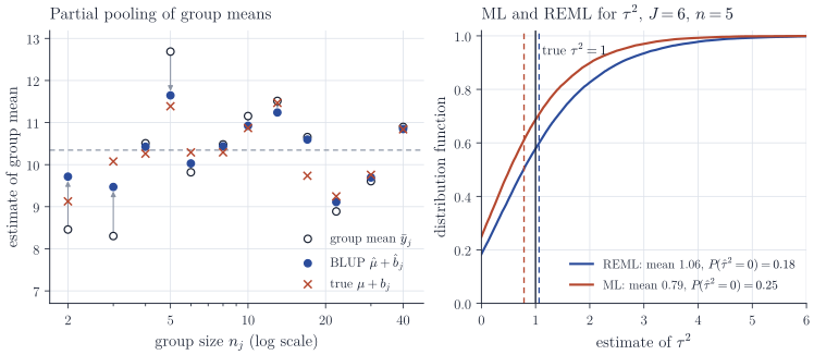
The plug-in step has a cost that the hierarchical view makes plain. Prediction intervals for \(b\) computed from \(\Var(b \mid y)\) at the estimated variance components treat those estimates as exact, and are too narrow when \(J\) is small; Kackar and Harville (1984, Journal of the American Statistical Association) quantified the resulting underestimation of mean squared error. A boundary estimate \(\hat\tau^2 = 0\), which the figure shows is common, sets every \(\lambda_j\) to zero and pools the groups completely.
Full Bayes
The third option gives \((\beta, \psi, \sigma^2)\) a prior and integrates over it. The posterior of \(b\) is then a mixture of the Gaussian posteriors of Theorem 1 over the posterior of the variance components, which propagates the uncertainty that plug-in methods ignore and avoids the boundary estimate, since the posterior of \(\tau\) is a distribution rather than a point. The REML connection suggests flat priors, and for \(\beta\) this is harmless. For the variance components it is not: the default prior \(\pi(\tau) \propto 1/\tau\) gives an improper posterior in this model for every data set, because the marginal likelihood of \(\tau\) stays positive as \(\tau \to 0\). Proper or weakly informative priors on the standard deviations, such as half-normal or half-\(t\) priors, are the usual remedy.
Remarks
The dictionary between the two vocabularies is short. Random effects are parameters with a Gaussian prior; the random-effects covariance \(G\) is the prior covariance; BLUP is the posterior mean under a flat prior on \(\beta\); Henderson’s equations are posterior mode equations, which is why they involve \(G^{-1}\) like a ridge penalty; ML and REML for variance components are type II maximum likelihood without and with integration over \(\beta\). The correspondence extends to generalized linear mixed models, where the integral over \(b\) is no longer Gaussian and the Laplace approximation used by standard software to integrate out \(b\) is the same approximation that Bayesians use for marginal likelihoods. Robinson (1991, Statistical Science) surveys BLUP from several points of view, including the Bayesian one.