Linear dimensionality reduction as optimization over orthonormal frames
Principal component analysis, Fisher’s discriminant analysis, canonical correlations, classical multidimensional scaling: textbooks usually present linear dimensionality reduction as a list of eigenvalue problems, one per method. Cunningham and Ghahramani (“Linear dimensionality reduction: survey, insights, and generalizations”, Journal of Machine Learning Research, 2015) proposed reading the list differently. Each method chooses a linear map to a lower dimension by optimizing an objective over a constraint set, and for a large family the constraint can be taken to be orthonormality of the projection. Seen this way, the eigenvector solution is a special property of a few objectives rather than the definition of the method, and objectives without such a solution can be optimized directly on the manifold of orthonormal frames. Below, PCA serves as the solvable case and a trace-ratio version of Fisher’s discriminant as a case without an eigenvector solution.
The framework
Let \(x_1, \dots, x_n \in \R^d\) be centred data and \(r < d\) the target dimension. A linear dimensionality reduction method returns \(M \in \R^{d \times r}\) and the reduced data \(y_i = M^\top x_i\). In the formulation considered here, \(M\) is restricted to the Stiefel manifold
\[\mathcal O^{d \times r} = \{M \in \R^{d \times r} : M^\top M = I_r\},\]and chosen as a maximizer of an objective \(f : \mathcal O^{d \times r} \to \R\) that depends on the data. The constraint has a clear meaning: \(MM^\top\) is the orthogonal projector onto the column space of \(M\), the reduced coordinates are coordinates of that projection in an orthonormal basis, and the scale of \(M\) cannot be inflated to improve the objective. It is a modelling choice, though, and the next sections show that it changes the answer for methods whose classical solutions are not orthonormal.
Many objectives depend on \(M\) only through its column space, that is, \(f(MQ) = f(M)\) for every orthogonal \(Q \in \R^{r \times r}\). They are then functions on the Grassmann manifold of \(r\)-dimensional subspaces, and the maximizer is a subspace, with any orthonormal basis of it equally good.
PCA: the solvable case
Let \(\Sigma = n^{-1}\sum_i x_ix_i^\top\) have eigenvalues \(\lambda_1 \ge \cdots \ge \lambda_d \ge 0\) and orthonormal eigenvectors \(u_1, \dots, u_d\). PCA can be defined by maximizing the retained variance or by minimizing the reconstruction error, and on the Stiefel manifold these coincide:
\[\frac1n\sum_{i=1}^n \lVert x_i - MM^\top x_i\rVert^2 = \tr\Sigma - \tr(M^\top \Sigma M),\]because \(I - MM^\top\) is an orthogonal projector, so \(\lVert x - MM^\top x\rVert^2 = x^\top x - x^\top MM^\top x\).
Theorem 1 (Ky Fan). For every \(M \in \mathcal O^{d\times r}\), \(\tr(M^\top\Sigma M) \le \lambda_1 + \cdots + \lambda_r\), with equality when the columns of \(M\) span \(\mathrm{span}\{u_1, \dots, u_r\}\). If \(\lambda_r > \lambda_{r+1}\), this is the only maximizing subspace.
Proof. Write \(\tr(M^\top\Sigma M) = \sum_{j=1}^d \lambda_j w_j\) with \(w_j = \lVert M^\top u_j\rVert^2 = u_j^\top MM^\top u_j\). Since \(MM^\top\) is an orthogonal projector of rank \(r\), \(0 \le w_j \le 1\) and \(\sum_j w_j = \tr(MM^\top) = r\). Using \(w_j \le 1\) for \(j \le r\) and \(\sum_{j \le r}(1 - w_j) = \sum_{j > r} w_j\),
\[\sum_{j=1}^d \lambda_j w_j \le \sum_{j \le r}\lambda_j - \lambda_r\sum_{j \le r}(1 - w_j) + \lambda_{r+1}\sum_{j > r} w_j = \sum_{j \le r}\lambda_j - (\lambda_r - \lambda_{r+1})\sum_{j > r} w_j ,\]which gives the bound, with equality when \(w_1 = \cdots = w_r = 1\). If \(\lambda_r > \lambda_{r+1}\), equality forces \(\sum_{j > r} w_j = 0\), hence \(w_1 = \cdots = w_r = 1\), so \(u_1, \dots, u_r\) lie in the column space of \(M\), which has dimension \(r\) and therefore equals their span.
Gradients on the Stiefel manifold and the PCA landscape
For a general objective one needs the first-order geometry of \(\mathcal O^{d \times r}\). Differentiating \(M(t)^\top M(t) = I_r\) along a smooth curve shows that the tangent space at \(M\) is
\[T_M = \{Z \in \R^{d \times r} : M^\top Z + Z^\top M = 0\} = \{M\Omega + (I - MM^\top)K : \Omega^\top = -\Omega,\ K \in \R^{d\times r}\}.\]With the Euclidean inner product \(\langle A, B\rangle = \tr(A^\top B)\) inherited from \(\R^{d \times r}\), the orthogonal projection onto \(T_M\) keeps the skew-symmetric part of \(M^\top G\) and the component of \(G\) orthogonal to the columns of \(M\):
\[P_M(G) = G - M\,\mathrm{sym}(M^\top G), \qquad \mathrm{sym}(A) = \tfrac12(A + A^\top).\]If \(f\) extends to a smooth function on a neighbourhood of the manifold with Euclidean gradient \(G = \nabla f(M)\), its Riemannian gradient is \(P_M(G)\), and a local maximizer must satisfy \(P_M(\nabla f(M)) = 0\). A gradient method moves along \(P_M(G)\) and returns to the manifold with a retraction, for instance the \(Q\) factor of a QR decomposition with positive diagonal in \(R\):
\[M_{k+1} = \mathrm{qf}\bigl(M_k + t_k P_{M_k}(\nabla f(M_k))\bigr).\]Edelman, Arias and Smith (“The geometry of algorithms with orthogonality constraints”, SIAM Journal on Matrix Analysis and Applications, 1998) and Absil, Mahony and Sepulchre, Optimization Algorithms on Matrix Manifolds, develop these tools, including second-order methods.
For PCA, \(f(M) = \tr(M^\top\Sigma M)\) has \(G = 2\Sigma M\), and since \(M^\top\Sigma M\) is symmetric,
\[P_M(2\Sigma M) = 2\bigl(\Sigma M - M (M^\top \Sigma M)\bigr).\]This vanishes exactly when \(\Sigma M = M(M^\top\Sigma M)\), that is, when the column space of \(M\) is invariant under \(\Sigma\). Under a gap condition every local maximum is global.
Proposition 2. Assume \(\lambda_1 > \cdots > \lambda_d\). The critical points of \(\tr(M^\top \Sigma M)\) on \(\mathcal O^{d\times r}\) are the orthonormal bases of the subspaces \(\mathrm{span}\{u_j : j \in S\}\), \(S \subseteq \{1, \dots, d\}\), \(\lvert S\rvert = r\). Every local maximum is global: it has \(S = \{1, \dots, r\}\).
Proof. With distinct eigenvalues, the \(\Sigma\)-invariant subspaces of dimension \(r\) are exactly the spans of \(r\) eigenvectors, which identifies the critical points. Suppose \(S \neq \{1, \dots, r\}\). Then there are \(i \in S\) and \(j \notin S\) with \(j < i\), so \(\lambda_j > \lambda_i\). Replace the basis vector \(u_i\) of the subspace by \(\cos t\, u_i + \sin t\, u_j\); the columns stay orthonormal, and the objective changes from \(\sum_{l \in S}\lambda_l\) by \(\sin^2 t\,(\lambda_j - \lambda_i) > 0\) for every small \(t \neq 0\). Since \(f\) depends only on the column space, this holds for every orthonormal basis of the subspace, so none of them is a local maximum.
This is the Stiefel-manifold counterpart of a classical result of Baldi and Hornik (“Neural networks and principal component analysis: learning from examples without local minima”, Neural Networks, 1989): the squared reconstruction error of a linear autoencoder with \(r\) hidden units, as a function of unconstrained encoder and decoder matrices, has no spurious local minima under a distinct-eigenvalue condition, and its global minima project onto the principal subspace. The absence of spurious local maxima is a property of this particular objective; for other objectives, gradient methods carry the usual risks of nonconvex optimization.
Fisher’s discriminant: two objectives, two answers
Suppose the data carry class labels, with within-class and between-class scatter matrices \(S_W \succ 0\) and \(S_B \succeq 0\), defined as the average within-class covariance and the covariance of the class means. A projection separates the classes well if, after projection, the between-class scatter is large relative to the within-class scatter. Two ways of making this precise are standard:
\[\text{ratio trace:}\ \ \tr\bigl((M^\top S_W M)^{-1} M^\top S_B M\bigr), \qquad \text{trace ratio:}\ \ f(M) = \frac{\tr(M^\top S_B M)}{\tr(M^\top S_W M)} .\]The ratio-trace criterion is invariant under \(M \mapsto MB\) for every invertible \(B\), so it depends only on the column space, and it is maximized by the leading generalized eigenvectors of \(S_Bv = \lambda S_Wv\), the classical solution. Those eigenvectors are \(S_W\)-orthogonal rather than orthogonal; orthonormalizing them keeps the subspace and hence the ratio-trace value. The trace ratio, which compares total between-class and total within-class scatter in an orthogonal projection, is the natural objective on the Stiefel manifold, and its maximizer is generally a different subspace. It has no closed form, but its optimal value has a one-dimensional characterization.
Proposition 3. Let \(\varphi(\rho) = \max_{M \in \mathcal O^{d\times r}} \tr\bigl(M^\top(S_B - \rho S_W)M\bigr)\), the sum of the \(r\) largest eigenvalues of \(S_B - \rho S_W\). Then \(\varphi\) is continuous and strictly decreasing, \(\rho_\star = \max_{\mathcal O^{d\times r}} f\) is its unique zero, and the maximizers of \(f\) are the \(M\) that attain \(\varphi(\rho_\star)\), that is, by Theorem 1, orthonormal bases of \(r\)-dimensional subspaces spanned by eigenvectors belonging to the \(r\) largest eigenvalues of \(S_B - \rho_\star S_W\).
Proof. The formula for \(\varphi\) is Theorem 1 applied to \(S_B - \rho S_W\) (Theorem 1 and its proof use only that the matrix is symmetric), and \(\rho_\star\) exists because \(f\) is continuous on the compact set \(\mathcal O^{d\times r}\). As a maximum of affine functions of \(\rho\), \(\varphi\) is convex, hence continuous; and for \(\rho < \rho'\), taking \(M'\) optimal at \(\rho'\), \(\varphi(\rho) \ge \varphi(\rho') + (\rho' - \rho)\tr(M'^\top S_W M') > \varphi(\rho')\) since \(S_W \succ 0\). Because \(\tr(M^\top S_W M) > 0\), the inequality \(f(M) \ge \rho\) is equivalent to \(\tr(M^\top(S_B - \rho S_W)M) \ge 0\). Hence \(\varphi(\rho) \ge 0\) if and only if \(\rho \le \rho_\star\), so \(\varphi(\rho_\star) = 0\), and \(f(M) = \rho_\star\) exactly when \(M\) attains \(\varphi(\rho_\star) = 0\).
Proposition 3 gives an exact solution by bisection on \(\rho\) with one symmetric eigendecomposition per step; iterative schemes of the same kind are standard in the trace-ratio literature. The framework’s generic route, Riemannian gradient ascent on \(f\) with the Euclidean gradient
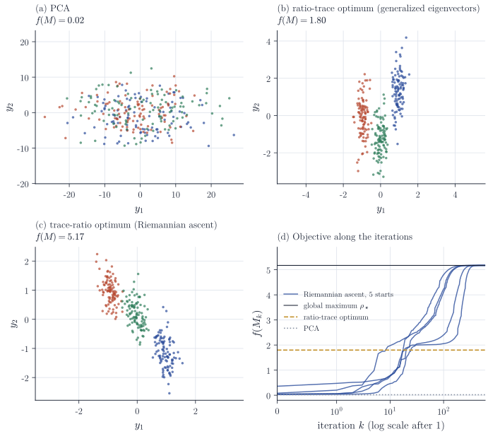
\[\nabla f(M) = \frac{2}{\tr(M^\top S_WM)}\Bigl(S_BM - f(M)\, S_W M\Bigr),\]needs no such structure. Figure 1 compares the three answers on simulated data with three classes in \(d = 6\) dimensions, where the directions of largest variance carry little class information. PCA finds those directions and separates almost nothing. The generalized eigenvectors separate the classes but are optimal for the ratio trace, not the trace ratio. Gradient ascent from five random orthonormal starts reaches the value \(\rho_\star\) computed from Proposition 3 in every run.
What the framework buys
Writing a method as “maximize \(f\) over \(\mathcal O^{d \times r}\)” separates two decisions that eigenvector formulations bundle together: what the projection should achieve, and how to compute it. Several consequences follow.
- Comparability. Methods become comparable through their objectives. PCA, Fisher-type discriminants and canonical correlations differ in \(f\) and, for canonical correlations, in having one projection for each of two sets of variables; classical multidimensional scaling with Euclidean distances is equivalent to PCA, computed through the Gram matrix.
- Generalization. A modified objective, such as a robust variance, a penalty encouraging sparse loadings, or a trace ratio in place of a ratio trace, needs a gradient rather than a new eigenvalue derivation.
- Heuristics made visible. When an objective has no eigenvector solution, orthonormalizing the eigenvectors of a related problem is a heuristic, and Figure 1 shows that it can be far from optimal for the criterion the projection is meant to serve.
The price is the usual one for nonconvex optimization: without results like Proposition 2 or Proposition 3, gradient methods guarantee only stationary points, and multiple starts or problem-specific analysis are needed. Cunningham and Ghahramani survey a larger set of methods that fit the framework and give the manifold optimization details; Absil, Mahony and Sepulchre is the standard reference for the algorithms.