The same p-value at every sample size: Lindley's paradox and the point null
Suppose a two-sided test of \(H_0 : \theta = \theta_0\) returns \(z = 1.96\), a p-value of 0.05. A frequentist reading of this result does not depend on the sample size: the data are exactly as surprising under \(H_0\) whether \(n = 20\) or \(n = 2 \times 10^6\). A Bayesian analysis with a prior probability on \(H_0\) reaches a conclusion that depends heavily on \(n\), and for large \(n\) it favours \(H_0\) overwhelmingly. Lindley (1957, Biometrika) made this conflict explicit, building on Jeffreys’s earlier work on significance tests; the phenomenon is often called the Jeffreys–Lindley paradox.
Set-up
Let \(X_1, \dots, X_n\) be independent \(N(\theta, \sigma^2)\) with \(\sigma > 0\) known, and write
\[z = \frac{\sqrt n \, (\bar X - \theta_0)}{\sigma}, \qquad r = \frac{n\tau^2}{\sigma^2}.\]The level-\(\alpha\) test rejects when \(\abs{z} > z_{\alpha/2}\), the upper \(\alpha/2\) quantile of \(N(0,1)\); the p-value is \(2\{1 - \Phi(\abs{z})\}\).
The Bayesian model puts probability \(\pi_0 \in (0, 1)\) on \(H_0\) and, under \(H_1\), spreads \(\theta\) according to \(N(\theta_0, \tau^2)\) with \(\tau > 0\). A point mass is needed: any continuous prior gives \(\{\theta = \theta_0\}\) probability zero before and after the data. Because \(\bar X\) is sufficient, the Bayes factor in favour of \(H_0\) is a ratio of two normal densities of \(\bar X\), namely \(N(\theta_0, \sigma^2/n)\) under \(H_0\) and, integrating \(\theta\) out, \(N(\theta_0, \tau^2 + \sigma^2/n)\) under \(H_1\):
\[B_{01} = \sqrt{\frac{\tau^2 + \sigma^2/n}{\sigma^2/n}} \, \exp\Bigl\{-\frac{(\bar X - \theta_0)^2}{2}\Bigl(\frac{n}{\sigma^2} - \frac{1}{\tau^2 + \sigma^2/n}\Bigr)\Bigr\}.\]Since \((\bar X - \theta_0)^2 n/\sigma^2 = z^2\) and \((\bar X - \theta_0)^2/(\tau^2 + \sigma^2/n) = z^2/(1 + r)\), this simplifies to
\[\begin{equation} B_{01} = \sqrt{1 + r} \, \exp\Bigl(-\frac{z^2}{2} \cdot \frac{r}{1 + r}\Bigr), \qquad \P(H_0 \mid X) = \Bigl(1 + \frac{1 - \pi_0}{\pi_0} \cdot \frac{1}{B_{01}}\Bigr)^{-1}. \label{eq:bf} \end{equation}\]The data enter only through \(z\), as for the classical test, and the sample size enters through \(r\).
The paradox
Proposition 1. Fix \(z\), \(\pi_0\), \(\tau\) and \(\sigma\). As \(n \to \infty\), \(B_{01} \to \infty\) and \(\P(H_0 \mid X) \to 1\). More precisely, \(B_{01} \ge \sqrt{1 + r}\, e^{-z^2/2}\) for all \(n\).
Proof. The exponent in \(\eqref{eq:bf}\) is at least \(-z^2/2\) because \(r/(1+r) < 1\), and \(\sqrt{1 + r} \to \infty\).
The same is true for any fixed p-value, however small. At \(z = 3.2905\) (p-value 0.001), \(\tau = \sigma\) and \(\pi_0 = 1/2\), the posterior probability of \(H_0\) exceeds one half once \(n \ge 50{,}380\); at \(z = 1.96\) this happens already for \(n \ge 42\) (Figure 1, left). The convergence need not be monotone: for small \(n\) the posterior probability first decreases (Figure 1). The result is a statement about the conditional evidence in a given \(z\), and it is not driven by the prior’s tails: the bound \(\sqrt{1 + r}\,e^{-z^2/2}\) grows like \(\tau\sqrt n/\sigma\) for any fixed \(\tau\).
The source of the behaviour is visible once the data are expressed on the scale of \(\theta\). A fixed \(z\) means \(\bar X - \theta_0 = z\sigma/\sqrt n\), so the likelihood concentrates on an interval of width of order \(\sigma/\sqrt n\) around a point that is itself only \(z\sigma/\sqrt n\) from \(\theta_0\). Every alternative at a fixed distance \(\delta \neq 0\) from \(\theta_0\) is eventually rejected by the data far more decisively than \(\theta_0\) is: its log likelihood ratio against \(\theta_0\) is
\[-\frac{n}{2\sigma^2}\bigl\{(\bar X - \theta_0 - \delta)^2 - (\bar X - \theta_0)^2\bigr\} = -\frac{n\delta^2}{2\sigma^2} + \frac{z\delta\sqrt n}{\sigma} \to -\infty .\]The alternatives that the data do support lie within \(O(\sigma/\sqrt n)\) of \(\theta_0\), and the \(N(\theta_0, \tau^2)\) prior gives them probability of order \(\sigma/(\tau\sqrt n)\). That factor is exactly \(1/\sqrt{1+r}\) up to constants. In this sense the Bayes factor charges \(H_1\) for the prior mass it wasted on values of \(\theta\) that the data rule out, and the charge grows without bound.
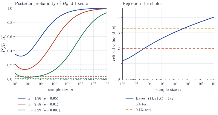
Two calibrations of the same statistic
Both procedures are functions of \(\abs z\), so they differ only in their thresholds. With \(\pi_0 = 1/2\) the Bayesian procedure prefers \(H_1\) when \(B_{01} < 1\), that is, when
\[z^2 > c_n^2 := \Bigl(1 + \frac1r\Bigr)\log(1 + r).\]Since \(r\) grows linearly in \(n\), \(c_n^2 = \log n + O(1)\): the Bayesian critical value grows like \(\sqrt{\log n}\), which is the same order as the penalty in the Bayesian information criterion. The implicit type I error rate of this rule can be computed from Mills’ ratio, \(1 - \Phi(c) \sim \varphi(c)/c\) as \(c \to \infty\). Because \(e^{-c_n^2/2} = (1 + r)^{-(1 + 1/r)/2} \sim r^{-1/2}\),
\[\alpha_n := \P_{\theta_0}(\abs{z} > c_n) \sim \frac{2\varphi(c_n)}{c_n} \sim \sqrt{\frac{2}{\pi}} \, \frac{\sigma}{\tau} \, \frac{1}{\sqrt{n \log n}} .\]A Bayesian who tests in this way therefore behaves like a frequentist whose significance level shrinks at the rate \((n \log n)^{-1/2}\). A frequentist who holds \(\alpha\) fixed behaves like a Bayesian whose prior mass on \(H_0\) shrinks with \(n\), or whose prior spread \(\tau\) shrinks like \(n^{-1/2}\). Neither choice is forced by logic; they reflect different questions. The fixed-level test controls the long-run frequency of false rejections at each \(n\). The Bayes factor compares how well the two hypotheses predicted the data actually observed.
The shrinking level has a consequence that classical tests lack.
Proposition 2. Let \(X_1, X_2, \dots\) be an infinite i.i.d. sequence and \(\P(H_0 \mid X)\) be computed from the first \(n\) observations. Under \(H_0\), \(\P(H_0 \mid X) \to 1\) almost surely. Under any fixed \(\theta \neq \theta_0\), \(\P(H_0 \mid X) \to 0\) almost surely.
Proof. Under \(H_0\), \(z = z_n = \sum_{i \le n}(X_i - \theta_0)/(\sigma\sqrt n)\), and the law of the iterated logarithm gives \(z_n^2 \le 3\log\log n\) for all large \(n\), almost surely. By the bound of Proposition 1, \(\log B_{01} \ge \tfrac12\log(1 + r) - \tfrac32\log\log n \to \infty\) almost surely, since \(r\) is proportional to \(n\). Under a fixed \(\theta \neq \theta_0\), the strong law gives \(z/\sqrt n \to (\theta - \theta_0)/\sigma\) almost surely, so
\[\log B_{01} = \tfrac12 \log(1 + r) - \frac{z^2}{2}\cdot\frac{r}{1+r} = \tfrac12 \log n - \frac{n(\theta - \theta_0)^2}{2\sigma^2}\bigl(1 + o(1)\bigr) + O(1) \to -\infty\]almost surely. In both cases the conclusion follows from \(\eqref{eq:bf}\).
A fixed-level test, by contrast, rejects a true null with probability \(\alpha\) at every \(n\). Whether this matters depends on what the point null represents.
How much can any prior favour the alternative?
One might hope that a better choice of prior under \(H_1\) would remove the conflict. It cannot remove it entirely. For any prior \(G\) on \(\theta\) under the alternative, the marginal density of \(\bar X\) under \(H_1\) is an average of \(N(\theta, \sigma^2/n)\) densities and is therefore at most the likelihood at \(\theta = \bar X\). Hence
\[B_{01}(G) \ge \frac{f(\bar X \mid \theta_0)}{\sup_\theta f(\bar X \mid \theta)} = e^{-z^2/2},\]with near-equality only for \(G\) concentrated at the observed \(\bar X\), a prior chosen after seeing the data. At \(z = 1.96\) this gives \(B_{01} \ge 0.146\) and, with \(\pi_0 = 1/2\), \(\P(H_0 \mid X) \ge 0.128\). A p-value of 0.05 thus corresponds to a posterior probability of the null of at least about 13% under every prior on the alternative, and typically much more. Bounds of this kind go back to Edwards, Lindman and Savage (1963, Psychological Review) and were developed by Berger and Sellke (1987, Journal of the American Statistical Association). The dashed lines in Figure 1 show \((1 + e^{z^2/2})^{-1}\) for the three values of \(z\).
The role of the prior variance
For fixed \(n\) and \(z\), letting \(\tau \to \infty\) also sends \(B_{01}\) to infinity, since \(r \to \infty\). A diffuse prior under the alternative is therefore not a neutral choice in testing; this is sometimes called Bartlett’s paradox. It is the reason improper priors cannot be used for the parameter that distinguishes the hypotheses: the Bayes factor inherits the arbitrary constant in the improper density. Default Bayes factors (Jeffreys’s Cauchy prior, intrinsic and fractional Bayes factors) are attempts to fix \(\tau\), or its analogue, on the scale of a single observation, which corresponds to \(\tau\) of order \(\sigma\) here.
Remarks
The paradox depends on taking the point null literally. If \(H_0\) stands for \(\abs{\theta - \theta_0} \le \varepsilon\), the point-mass approximation is accurate only while \(\varepsilon\) is small compared with \(\sigma/\sqrt n\), the resolution of the experiment. Berger and Delampady (1987, Statistical Science) analyse when this approximation is reasonable. For very large \(n\) it eventually fails, and an interval null then behaves differently. Conversely, if the point null is a genuine scientific possibility, such as a conservation law or a treatment with no mechanism of action, then the posterior probability answers a question that the p-value does not address. The underlying disagreement is about what a test is for, and the elementary formula \(\eqref{eq:bf}\) makes the terms of that disagreement precise. Jeffreys’s Theory of Probability and Lindley’s 1957 paper remain the primary sources; Robert, The Bayesian Choice, discusses the paradox alongside default Bayes factors.