Slicing the range instead of the domain: a picture of the Lebesgue integral

October 12, 2026Probability

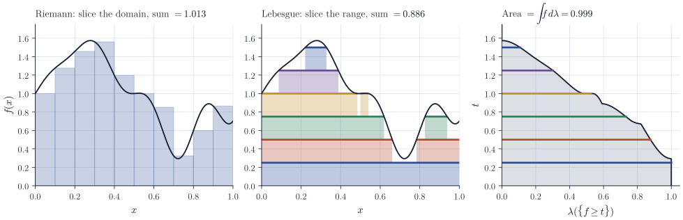
A Riemann sum approximates the area under a graph by vertical strips: cut the domain into small intervals and multiply each width by a value of the function on it. The approximation is good when the function varies little on each interval, so its quality is governed by the regularity of \(f\) as a function of \(x\). The Lebesgue integral cuts the other axis. Choose levels \(0 < y_1 < y_2 < \cdots\), and for each level measure the set of points where \(f\) is at least that high. The pieces are horizontal slabs, whose bases can be arbitrary measurable sets rather than intervals. Nothing about the arrangement of these sets matters, only their size, which is why the construction works on any measure space and for functions with no regularity at all.

Throughout, \((\mathcal X, \mathcal A, \mu)\) is a measure space and \(f : \mathcal X \to [0, \infty]\) is measurable.

Definition through simple functions

A simple function is a finite combination \(\varphi = \sum_{j=1}^m a_j\mathbf 1_{A_j}\) with \(a_j \ge 0\) and \(A_j \in \mathcal A\); its integral is \(\int\varphi\,\dd\mu = \sum_j a_j\,\mu(A_j)\), which does not depend on the representation. For measurable \(f \ge 0\) one defines

\[\int f\,\dd\mu = \sup\Bigl\{\int\varphi\,\dd\mu : \varphi \text{ simple},\ 0 \le \varphi \le f\Bigr\}.\]

Two facts from the standard development are used below: the integral is monotone, and the monotone convergence theorem holds: if \(0 \le g_1 \le g_2 \le \cdots\) are measurable and \(g_n \uparrow g\) pointwise, then \(\int g_n\,\dd\mu \uparrow \int g\,\dd\mu\).

Dyadic slicing

The supremum in the definition is the limit along an explicit sequence of simple functions that slices the range of \(f\) at the dyadic levels \(k2^{-n}\). For \(n \ge 1\) let

\[\varphi_n = \min\bigl(n,\ 2^{-n}\lfloor 2^n f\rfloor\bigr) = \sum_{k=1}^{n2^n} 2^{-n}\,\mathbf 1\{f \ge k2^{-n}\}.\]

The two expressions agree because, at a point where \(f(x) = s\), the sum counts the levels \(k2^{-n} \le \min(s, n)\), and there are exactly \(\min(n2^n, \lfloor 2^ns\rfloor)\) of them. The second expression is the horizontal-slab picture: \(\varphi_n\) stacks slabs of height \(2^{-n}\) whose bases are the superlevel sets \(\{f \ge k2^{-n}\}\), which are measurable because \(f\) is.

Lemma 1. Each \(\varphi_n\) is simple, \(\varphi_n \le \varphi_{n+1} \le f\), and \(\varphi_n \to f\) pointwise. Moreover \(0 \le f - \varphi_n \le 2^{-n}\) on \(\{f < n\}\).

Proof. Simplicity is clear from the second expression. For a real number \(s \ge 0\), \(2^{-n}\lfloor 2^ns\rfloor \le s < 2^{-n}\lfloor 2^ns\rfloor + 2^{-n}\); this gives \(\varphi_n \le f\) and the error bound on \(\{f < n\}\). For monotonicity in \(n\), note that \(\lfloor 2a\rfloor \ge 2\lfloor a\rfloor\) for \(a \ge 0\), so \(2^{-n}\lfloor 2^ns\rfloor \le 2^{-(n+1)}\lfloor 2^{n+1}s\rfloor\); taking minima with the caps \(n \le n + 1\) preserves the inequality. Pointwise convergence follows from the error bound where \(f < \infty\), and from \(\varphi_n = n\) where \(f = \infty\).

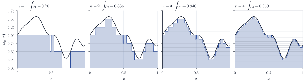
By the monotone convergence theorem, \(\int\varphi_n\,\dd\mu \uparrow \int f\,\dd\mu\). Figure 2 below shows the first four approximations for a function on \([0, 1]\); each refinement halves the slab height and fills in the space under the graph from below.

The integral as an integral of the distribution function

The integral of \(\varphi_n\) is a sum over levels:

\[\int\varphi_n\,\dd\mu = \sum_{k=1}^{n2^n}2^{-n}\,G\bigl(k2^{-n}\bigr), \qquad G(t) = \mu(\{f \ge t\}).\]

The function \(G : (0, \infty) \to [0, \infty]\) is nonincreasing, so this is a Riemann sum for \(G\) on \([0, n]\) with mesh \(2^{-n}\), evaluated at right endpoints. Because \(G\) is monotone, the Riemann sums can be compared with integrals of \(G\) from both sides, and passing to the limit gives the following representation, often called the layer cake formula.

Theorem 2. For every measurable \(f : \mathcal X \to [0, \infty]\),

\[\int f\,\dd\mu = \int_0^\infty \mu(\{f \ge t\})\,\dd t,\]

where the right-hand side is the Lebesgue integral on \((0, \infty)\) of the nonincreasing function \(G\), possibly infinite. The same holds with \(\{f > t\}\) in place of \(\{f \ge t\}\).

Proof. Write \(t_k = k2^{-n}\). Since \(G\) is nonincreasing, \(G(t_k) \le G(t)\) for \(t \in (t_{k-1}, t_k]\), and \(G(t) \le G(t_k)\) for \(t \in [t_k, t_{k+1})\). Integrating these inequalities over the intervals and summing,

\[\int_{2^{-n}}^{n} G(t)\,\dd t \le \sum_{k=1}^{n2^n - 1}2^{-n}G(t_k) \le \int\varphi_n\,\dd\mu \le \sum_{k=1}^{n2^n}\int_{t_{k-1}}^{t_k}G(t)\,\dd t \le \int_0^\infty G(t)\,\dd t .\]

As \(n \to \infty\), the left-hand side increases to \(\int_0^\infty G\), the right-hand side, by monotone convergence applied to \(G\,\mathbf 1_{[2^{-n}, n]}\). Hence \(\int\varphi_n\,\dd\mu \to \int_0^\infty G\), while \(\int\varphi_n\,\dd\mu \to \int f\,\dd\mu\) by Lemma 1 and monotone convergence.

For the strict version, let \(G_>(t) = \mu(\{f > t\})\). Then \(G(t + \varepsilon) \le G_>(t) \le G(t)\) for \(\varepsilon > 0\), so \(\int_0^\infty G(t + \varepsilon)\,\dd t = \int_\varepsilon^\infty G \le \int_0^\infty G_> \le \int_0^\infty G\), and letting \(\varepsilon \downarrow 0\) gives equality by monotone convergence.

No finiteness or \(\sigma\)-finiteness of \(\mu\) was needed. The theorem says that the Lebesgue integral of \(f\) is the area under the curve \(t \mapsto \mu(f \ge t)\), and Figure 1 draws exactly this. The left panel is a Riemann sum with ten intervals. The middle panel is the Lebesgue sum with levels spaced \(1/4\) apart: each coloured segment is the superlevel set \(\{f \ge k/4\}\), and below it a slab of height \(1/4\). The right panel turns the picture on its side: plotting the length of each superlevel set against its level traces out \(G\), the coloured segments become the terms of the Riemann sum for \(G\), and the shaded area is \(\int f\).

Figure 1. The function $f(x) = 1 + \frac12\sin(2\pi x) + 0.3\,x\cos(7\pi x)$ on $[0,1]$. Left: left-endpoint Riemann sum with ten intervals. Middle: Lebesgue sum with levels $k/4$; the segment at height $k/4$ is the set $\{f \ge k/4\}$, which may consist of several intervals. Right: $t \mapsto \lambda(\{f \ge t\})$ with the same levels marked; the area under this curve equals $\int_0^1 f\,d\lambda$.

Figure 2. The dyadic approximations $\varphi_n = \min(n, 2^{-n}\lfloor 2^n f\rfloor)$ for $n = 1, \dots, 4$, with the levels $k2^{-n}$ drawn as horizontal lines; for $n = 1$ the cap at height one is visible. The integrals increase to $\int_0^1 f\,d\lambda \approx 0.999$.

What slicing the range buys

Error control without regularity. If \(0 \le f \le M\) and \(\mu(\{f > 0\}) < \infty\), then for \(n \ge M\) Lemma 1 gives

\[0 \le \int f\,\dd\mu - \int\varphi_n\,\dd\mu \le 2^{-n}\,\mu(\{f > 0\}),\]

since \(f - \varphi_n\) is at most \(2^{-n}\) and vanishes outside \(\{f > 0\}\). The bound involves only the range of \(f\) and the size of its support, not how wildly \(f\) oscillates in \(x\). For a Riemann sum the error is controlled by the oscillation of \(f\) over each subinterval, and it need not go to zero at all.

Functions without Riemann integrals. The indicator of the rationals in \([0,1]\) has Riemann sums equal to \(0\) or \(1\) depending on whether the tags are irrational or rational, so it is not Riemann integrable; its Lebesgue integral is \(\lambda(\mathbb Q \cap [0,1]) = 0\). A less degenerate example is the indicator of a fat Cantor set \(C \subset [0,1]\), built like the middle-thirds set but removing at stage \(j\) the open middle intervals of length \(4^{-j}\) from each of the \(2^{j-1}\) remaining intervals. The removed length is \(\sum_{j\ge1}2^{j-1}4^{-j} = 1/2\), so \(\lambda(C) = 1/2\), and \(C\) contains no interval. Every point of \(C\) is therefore a limit of points outside \(C\), so \(\mathbf 1_C\) is discontinuous on a set of measure \(1/2\). By Lebesgue’s criterion, a bounded function on a compact interval is Riemann integrable if and only if its set of discontinuities has measure zero, so \(\mathbf 1_C\) has no Riemann integral, while its Lebesgue integral is \(1/2\), read off from a single slab. When the Riemann integral does exist, the two integrals agree.

Expectations. On a probability space, Theorem 2 is the familiar tail formula for a nonnegative random variable,

\[\E X = \int_0^\infty \P(X > t)\,\dd t,\]

and applying it to \(X^p\) with the substitution \(t = s^p\) gives \(\E X^p = \int_0^\infty p\,s^{p-1}\,\P(X > s)\,\dd s\) for \(p > 0\). These identities turn tail bounds into moment bounds, and they hold whether \(X\) is discrete, continuous or neither, because the right-hand side only involves the distribution function of \(X\).

Remarks

Lebesgue’s construction integrates more functions than Riemann’s, but its main advantage is that integrals behave well under limits: the monotone and dominated convergence theorems hold in full generality, and spaces such as \(L^p\) are complete. The slicing picture is the reason the theory needs nothing from the domain except a measure: horizontal slabs only require the measure of superlevel sets.

G. B. Folland, Real Analysis, develops the integral from simple functions as above and proves Lebesgue’s criterion for Riemann integrability. E. H. Lieb and M. Loss, Analysis, use the layer cake representation systematically, for instance in the theory of symmetric decreasing rearrangements.