Just-in-time compilation in JAX: tracing, fusion and where the time goes

October 12, 2026Computation

Most methodological work in statistics ends with an algorithm, and most algorithms end up as code in an interpreted language. How fast that code runs is rarely discussed, yet it decides which experiments are feasible: a simulation study with \(10^4\) replications of an MCMC run of \(10^5\) iterations is a different proposition at one microsecond per iteration than at a hundred. The sections below look at where the time goes in numerical Python, what just-in-time (JIT) compilation does about it, and what it costs, with JAX as the concrete system.

Two sources of overhead

NumPy makes array code fast by moving loops out of the interpreter into compiled C. A call such as np.exp(x) runs one compiled loop over the elements of x. Two costs remain.

The first is a fixed cost per operation. Before the loop starts, the interpreter executes the bytecode of the call, NumPy checks argument types and shapes, selects a compiled kernel for the data type and allocates an output array. On current hardware this is of the order of a microsecond, independent of the array length.

The second is memory traffic. The expression

np.sum(np.exp(-0.5 * x**2) * np.cos(3 * x) + x * np.tanh(x))

consists of about ten operations, each of which reads one or two full arrays and writes a new temporary array. For long arrays the arithmetic is cheap compared with moving the data, and the expression makes ten passes over memory where one would do.

A crude model for an expression with \(k\) operations on arrays of length \(n\) is therefore

\[\text{time} \approx k\,(c_0 + c_1 n),\]

with \(c_0\) the fixed cost and \(c_1\) the per-element cost of one pass. For small \(n\) the fixed costs dominate; for large \(n\) the \(k\) passes do. Loops whose iterations depend on each other, such as Markov chains, filters and recursive simulations, cannot be vectorized at all. Each iteration then executes a handful of scalar operations and pays \(c_0\) for each, so the interpreter, and not the arithmetic, sets the speed.

What jax.jit does

A JIT compiler compiles code at run time, when the types and shapes of the inputs are known. In JAX this happens in three stages.

Tracing. When a function decorated with jax.jit is called, JAX calls the Python function once with abstract arguments that carry only a shape and a data type. Every jax.numpy operation applied to such a tracer is recorded instead of executed. The result is a jaxpr, a small typed intermediate language. For the expression above and an input of length \(5\) in double precision, JAX 0.11 prints

{ lambda ; a:f64[5]. let
    b:f64[5] = integer_pow[y=2] a
    c:f64[5] = mul -0.5:f64[] b
    d:f64[5] = exp c
    e:f64[5] = mul 3.0:f64[] a
    f:f64[5] = cos e
    g:f64[5] = mul d f
    h:f64[5] = tanh a
    i:f64[5] = mul a h
    j:f64[5] = add g i
    k:f64[] = reduce_sum[axes=(0,) out_sharding=None] j
  in (k,) }

The Python code has disappeared; what remains is a straight-line program of primitive operations on arrays of known shape.

Compilation. The jaxpr is handed to XLA, an optimizing compiler for array programs, which generates machine code for the target device. Among its optimizations, the most important here is fusion: the nine elementwise operations and the reduction become a single loop that reads each \(x_i\) once, computes the summand in registers and accumulates it, with no temporary arrays.

Caching. The compiled code is cached under a key that includes the shapes and data types of the arguments. Later calls with the same signature skip tracing and compilation and run the machine code directly, at a fixed cost of a few microseconds per call. A call with a new shape triggers a new trace and compilation.

The price: what may appear inside a compiled function

Tracing explains every restriction that JAX imposes.

• Python control flow is executed during tracing, when only shapes are known. A condition such as if x[0] > 0: on a traced value therefore raises an error; data-dependent branches must be written with jnp.where or jax.lax.cond. A Python for loop is allowed but is unrolled into the jaxpr, so a loop of \(10^5\) steps produces a program of \(10^5\) copies of its body. Long loops should use jax.lax.fori_loop or jax.lax.scan, which compile the body once.
• Side effects happen once, at tracing time. A print inside a jitted function prints a tracer on the first call and nothing afterwards.
• Functions must be pure. In particular there is no global random state: random numbers are drawn from explicit keys, jax.random.normal(key, shape), and fresh keys are produced with jax.random.split. This makes the randomness of a computation an explicit argument, which is good practice in any case.
• JAX uses single precision by default. Statistical code usually needs jax.config.update("jax_enable_x64", True), which all timings below use.

A sequential recursion such as \(x_t = \tanh(0.9\, x_{t-1}) + e_t\) becomes

def step(x, e_t):
    x = jnp.tanh(0.9 * x) + e_t
    return x, x                      # (carry, output)

simulate = jax.jit(lambda e: jax.lax.scan(step, 0.0, e)[1])

lax.scan compiles step once and runs the loop in machine code, so the interpreter is involved only in the initial call.

Measurements

Figure 1 compares the approaches on two problems. All timings were measured once by the Python figure script on a two-core Intel Xeon virtual machine at 2.1 GHz, in double precision, and written to a data file that the R and Julia versions of the figure also read; they are specific to this machine and to JAX 0.11.2 and NumPy 2.5. Each point is the smallest time per call over several batches of repeated calls, after a warm-up call, and JAX results are synchronized with block_until_ready() before the clock stops. The last detail matters: JAX dispatches work asynchronously, and timing a call without blocking measures only the time to enqueue it.

Figure 1. Left: time per call of the elementwise expression above as a function of the array length, for NumPy, for JAX executing one operation at a time, and for the jit-compiled function; the dashed line is the first call of a freshly jitted function, which includes tracing and compilation. 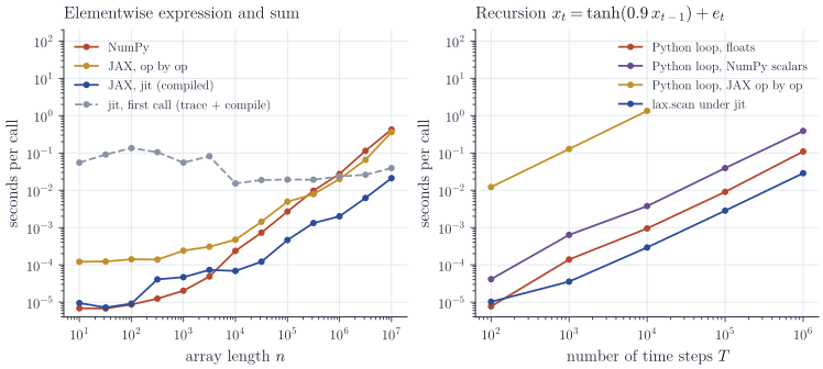Right: time to simulate $T$ steps of the recursion with a Python loop over floats, a Python loop over NumPy scalars, a Python loop over JAX operations, and lax.scan under jit.

Short arrays. For \(n \le 100\), NumPy and the compiled function both take about \(7\) to \(9\) microseconds per call: fixed costs dominate and compilation has nothing to remove. JAX without jit takes about \(120\) microseconds, because each of its operations has a larger dispatch cost than NumPy’s. For intermediate lengths, roughly \(300\) to \(3{,}000\), the compiled function was slower than NumPy on this machine (about \(41\) against \(12\) microseconds at \(n = 316\)); the cause was not investigated, and the example is a reminder that the crude model above is no substitute for measurement.

Long arrays. At \(n = 10^5\) the compiled function takes \(0.46\) milliseconds against \(2.7\) for NumPy, and at \(n = 10^7\) it takes \(21\) milliseconds against \(424\). Fusion removes the temporaries and the repeated passes, but this benchmark does not isolate it: XLA also uses its own vectorized implementations of exp, cos and tanh and may divide large loops between the two cores. Compilation does not change the arithmetic in any important way: for standard normal inputs the summands computed by the compiled function and by NumPy differed by less than \(2 \times 10^{-15}\).

Compilation cost. The first call of a new jitted function took between \(15\) and \(135\) milliseconds. If an interpreted implementation takes \(t_I\) per call and the compiled one \(t_J < t_I\) after a compilation cost \(C\), then \(m\) calls cost \(m t_I\) and \(C + m t_J\) respectively, and compilation pays off once

\[m > \frac{C}{t_I - t_J}.\]

At \(n = 10^5\), with \(C \approx 19\) milliseconds and a saving of about \(2.2\) milliseconds per call, that is after about nine calls. Inside an optimizer, a sampler or a simulation study, where the same function is evaluated thousands of times on inputs of fixed shape, the compilation cost is negligible. In interactive work on inputs of changing shape it may dominate.

Sequential loops. For the recursion, the compiled scan needs about \(29\) nanoseconds per step at \(T = 10^6\), against \(109\) for a Python loop over floats and \(388\) for a Python loop over NumPy scalars, whose per-operation overhead exceeds that of plain floats. A Python loop over JAX operations is the worst choice by far, at about \(130\) microseconds per step, since every step pays JAX’s dispatch cost several times. The gain from scan here is smaller than in the elementwise case because each step is a dependent scalar computation that no compiler can vectorize.

Remarks

JIT compilation composes with JAX’s other transformations: jax.grad produces a new function whose jaxpr computes derivatives, and jax.vmap vectorizes a function over a batch axis, so that, for example, many independent chains of a sampler can be compiled into one program. The same idea appears elsewhere in different forms. Numba compiles Python functions over NumPy arrays and scalars with LLVM and handles explicit loops well; Julia is designed around JIT compilation, specializing every function on the concrete types of its arguments (Bezanson, Edelman, Karpinski and Shah, “Julia: a fresh approach to numerical computing”, SIAM Review, 2017). The design of JAX’s tracing approach is described by Frostig, Johnson and Leary, “Compiling machine learning programs via high-level tracing” (SysML, 2018). Whatever the system, two habits carry over: measure steady-state time separately from compilation time, and make sure the clock stops only after the computation has finished.