Shrinking unrelated means: Stein’s identity and the James–Stein estimator

Suppose we observe $X = (X_1, \dots, X_p)$ with $X \sim N_p(\theta, I_p)$ and want to estimate the whole vector $\theta$ under the loss $\lVert \hat\theta - \theta \rVert^2 = \sum_i (\hat\theta_i - \theta_i)^2$. The coordinates are independent and each $X_i$ carries information only about $\theta_i$, so the estimator $\hat\theta = X$ looks unimprovable. It is the maximum likelihood estimator, it is unbiased, its risk $\E_\theta \lVert X - \theta \rVert^2 = p$ does not depend on $\theta$, and it is minimax. Stein (1956) showed that it is nevertheless inadmissible when $p \ge 3$, and James and Stein (1961) gave an explicit estimator with uniformly smaller risk:

\[\hat\theta^{\mathrm{JS}} = \Bigl(1 - \frac{p - 2}{\lVert X \rVert^2}\Bigr) X .\]

A heuristic explains the direction of the improvement. Since $\E \lVert X \rVert^2 = \lVert \theta \rVert^2 + p$, the observed vector is systematically longer than the target, and pulling it back toward the origin by an amount estimated from the data can reduce the error on average. Whether it does so for every $\theta$ is a question about exact risks, and the answer rests on one identity.

Stein’s identity

Lemma 1 (Stein). Let $Z \sim N(\mu, 1)$ and let $h : \R \to \R$ be absolutely continuous with $\E \abs{h'(Z)} < \infty$. Then $\E\abs{(Z - \mu) h(Z)} < \infty$ and $\E[(Z - \mu) h(Z)] = \E[h'(Z)]$.

Proof. Let $\varphi$ be the $N(\mu, 1)$ density. Since $\varphi'(t) = -(t - \mu)\varphi(t)$ and $\varphi$ vanishes at $\pm\infty$,

\[\varphi(x) = \int_x^\infty (t - \mu) \varphi(t) \, \dd t \quad (x \ge \mu), \qquad \varphi(x) = -\int_{-\infty}^x (t - \mu) \varphi(t) \, \dd t \quad (x \le \mu).\]

Substituting into $\E h'(Z) = \int h'(x) \varphi(x) \, \dd x$ and exchanging the order of integration,

\[\begin{aligned} \E h'(Z) &= \int_\mu^\infty (t - \mu)\varphi(t) \Bigl(\int_\mu^t h'(x)\, \dd x\Bigr) \dd t + \int_{-\infty}^\mu (t - \mu)\varphi(t) \Bigl(-\int_t^\mu h'(x)\, \dd x\Bigr) \dd t \\ &= \E\bigl[(Z - \mu)\bigl(h(Z) - h(\mu)\bigr)\bigr]. \end{aligned}\]

Fubini’s theorem applies because the same computation with $\abs{h'}$ in place of $h'$ gives the finite value $\E \abs{h'(Z)}$, and it also shows $\E\abs{(Z - \mu)(h(Z) - h(\mu))} \le \E\abs{h'(Z)}$. Finally $\E(Z - \mu) h(\mu) = 0$.

For $X \sim N_p(\theta, I_p)$ and $g : \R^p \to \R^p$, apply the lemma to the $i$-th coordinate conditionally on the others. If for almost every value of $(x_j)_{j \ne i}$ the function $x_i \mapsto g_i(x)$ is absolutely continuous, and $\E \abs{\partial_i g_i(X)} < \infty$, then $\E[(X_i - \theta_i) g_i(X)] = \E[\partial_i g_i(X)]$. Summing over $i$,

\[\E\bigl[(X - \theta)^\top g(X)\bigr] = \E\bigl[\nabla \cdot g(X)\bigr] . \tag{1}\]

Unbiased risk estimation

Write a candidate estimator as $\hat\theta = X + g(X)$. Expanding the square,

\[\lVert X + g(X) - \theta \rVert^2 = \lVert X - \theta \rVert^2 + \lVert g(X) \rVert^2 + 2 (X - \theta)^\top g(X),\]

and taking expectations with (1), provided $\E \lVert g(X) \rVert^2 < \infty$ and the conditions for (1) hold,

\[\E_\theta \lVert \hat\theta - \theta \rVert^2 = \E_\theta\Bigl[ p + \lVert g(X) \rVert^2 + 2\, \nabla \cdot g(X) \Bigr] .\]

The quantity in brackets, $\mathrm{SURE}(X) = p + \lVert g(X) \rVert^2 + 2 \nabla \cdot g(X)$, depends on the data only, so it is an unbiased estimator of the risk at every $\theta$. This is Stein’s unbiased risk estimate. It is useful far beyond the present problem, for instance for choosing smoothing parameters, and here it makes the James–Stein calculation immediate.

The James–Stein estimator

Take $g(x) = -c\, x / \lVert x \rVert^2$ for a constant $c > 0$. For $x \ne 0$,

\[\partial_i \frac{x_i}{\lVert x \rVert^2} = \frac{1}{\lVert x \rVert^2} - \frac{2 x_i^2}{\lVert x \rVert^4}, \qquad \nabla \cdot \frac{x}{\lVert x \rVert^2} = \frac{p - 2}{\lVert x \rVert^2}, \qquad \Bigl\lVert \frac{x}{\lVert x \rVert^2} \Bigr\rVert^2 = \frac{1}{\lVert x \rVert^2} .\]

The conditions for (1) hold when $p \ge 3$: the function is smooth in $x_i$ whenever the other coordinates are not all zero, the partial derivatives are bounded in absolute value by $1 / \lVert x \rVert^2$, and $\E\, \lVert X \rVert^{-2} < \infty$ (shown below). Hence

\[R(\theta, X + g(X)) = p - \bigl(2c(p - 2) - c^2\bigr)\, \E_\theta \frac{1}{\lVert X \rVert^2} .\]

The coefficient $2c(p-2) - c^2$ is positive for $0 < c < 2(p - 2)$ and maximal at $c = p - 2$, which gives the James–Stein estimator.

Theorem 2. For $p \ge 3$ and every $\theta \in \R^p$,

\[R(\theta, \hat\theta^{\mathrm{JS}}) = p - (p - 2)^2\, \E_\theta \frac{1}{\lVert X \rVert^2} = p - (p - 2)^2\, \E\Bigl[\frac{1}{p - 2 + 2K}\Bigr],\]

where $K \sim \mathrm{Poisson}\bigl(\lVert \theta \rVert^2 / 2\bigr)$. In particular $R(\theta, \hat\theta^{\mathrm{JS}}) < p$ for every $\theta$, $R(0, \hat\theta^{\mathrm{JS}}) = 2$, and $R(\theta, \hat\theta^{\mathrm{JS}}) \le p - (p - 2)^2 / (p - 2 + \lVert \theta \rVert^2)$.

Proof. The first equality is the display before the theorem with $c = p - 2$. For the second, $\lVert X \rVert^2$ has the noncentral chi-squared distribution with $p$ degrees of freedom and noncentrality $\lambda = \lVert \theta \rVert^2$, which is the mixture of central $\chi^2_{p + 2K}$ distributions with $K \sim \mathrm{Poisson}(\lambda/2)$. For a central $\chi^2_m$ variable with $m > 2$,

\[\E \frac{1}{\chi^2_m} = \int_0^\infty \frac{1}{u} \cdot \frac{u^{m/2 - 1} e^{-u/2}}{2^{m/2} \Gamma(m/2)} \, \dd u = \frac{2^{m/2 - 1} \Gamma(m/2 - 1)}{2^{m/2} \Gamma(m/2)} = \frac{1}{m - 2},\]

and conditioning on $K$ gives $\E_\theta \lVert X \rVert^{-2} = \E[1/(p - 2 + 2K)] \le 1/(p - 2) < \infty$. At $\theta = 0$, $K = 0$ and the risk is $p - (p - 2) = 2$. The final bound is Jensen’s inequality for the convex function $k \mapsto 1/(p - 2 + 2k)$, with $\E(2K) = \lVert \theta \rVert^2$.

The gain is largest near the shrinkage target and disappears as $\lVert \theta \rVert \to \infty$, where the shrinkage factor tends to one. It is also larger in higher dimension: at $\theta = 0$ the risk is $2$ whatever $p$ is, so the relative risk $2/p$ tends to zero.

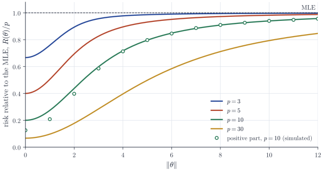
Risk of the James-Stein estimator divided by p, as a function of the norm of theta, for p equal to 3, 5, 10 and 30, with simulated risk of the positive-part estimator for p equal to 10. — Figure 1. Exact risk of $\hat\theta^{\mathrm{JS}}$ relative to the risk $p$ of the MLE, from the Poisson mixture formula of Theorem 2. Circles: Monte Carlo risk of the positive-part estimator for $p = 10$ ($40{,}000$ replications per point), which is visibly smaller near the origin.

When $\lVert X \rVert^2 < p - 2$ the shrinkage factor $1 - (p-2)/\lVert X \rVert^2$ is negative, and the estimator flips the sign of $X$, which is hard to defend. The positive-part estimator $\bigl(1 - (p - 2)/\lVert X \rVert^2\bigr)_+ X$ truncates the factor at zero and has uniformly smaller risk than $\hat\theta^{\mathrm{JS}}$; a proof is in Lehmann and Casella, Theory of Point Estimation. It is itself inadmissible: by a theorem of Brown (1971, Annals of Mathematical Statistics), every admissible estimator in this problem is generalized Bayes and hence a real-analytic function of $X$, which the positive-part estimator is not on the sphere $\lVert X \rVert^2 = p - 2$. The improvements available over it are small, however.

An empirical Bayes reading

The estimator becomes natural under a prior. If $\theta_1, \dots, \theta_p$ are i.i.d. $N(0, \tau^2)$, the posterior mean is $(1 - B) X$ with $B = 1/(1 + \tau^2)$, and its Bayes risk is $p(1 - B)$. The variance $\tau^2$ is unknown, but it can be estimated from the data, because marginally $X_i \sim N(0, 1 + \tau^2)$ independently, so $\lVert X \rVert^2 / (1 + \tau^2) \sim \chi^2_p$ and

\[\E\Bigl[\frac{p - 2}{\lVert X \rVert^2}\Bigr] = \frac{p - 2}{(1 + \tau^2)(p - 2)} = B .\]

The James–Stein estimator is the posterior mean with $B$ replaced by this unbiased estimate. Averaging Theorem 2 over the prior gives its Bayes risk exactly: $p - (p - 2)^2 \E[1/\lVert X \rVert^2] = p - (p - 2) B$, which exceeds the Bayes risk $p - pB$ of the oracle posterior mean by only $2B \le 2$. The data from all coordinates are used to estimate how much to shrink, and this is how the apparently unrelated coordinates inform each other; Efron and Morris developed this interpretation.

Choosing the target

Nothing singles out the origin. Shrinking toward any fixed point $\theta_0$ gives the same risk function with $\theta$ replaced by $\theta - \theta_0$. More usefully, one can shrink toward the grand mean $\bar X$. Write $X = \bar X \mathbf 1 + (X - \bar X \mathbf 1)$. The first component is the projection onto the span of $\mathbf 1$, and in an orthonormal basis adapted to this decomposition the second component is a $N_{p-1}$ vector with identity covariance. Leaving the first component alone and applying James–Stein to the second gives, for $p \ge 4$,

\[\hat\theta^{\mathrm{JS}, \bar X} = \bar X \mathbf 1 + \Bigl(1 - \frac{p - 3}{S}\Bigr)(X - \bar X \mathbf 1), \qquad S = \sum_{i=1}^p (X_i - \bar X)^2 ,\]

with risk $1 + \bigl[(p - 1) - (p - 3)^2 \E(1/S)\bigr] = p - (p - 3)^2\, \E(1/S)$, by Theorem 2 in dimension $p - 1$. The gain now depends on the spread $\sum_i (\theta_i - \bar\theta)^2$ rather than on $\lVert \theta \rVert^2$, so it is large whenever the means are similar to each other, wherever they are located.

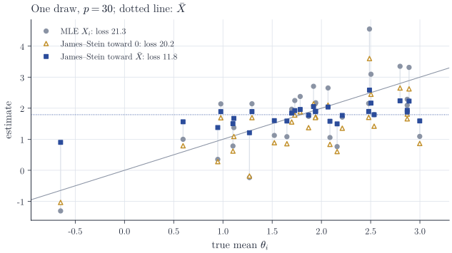
Scatter plot of estimates against true means for the MLE and two James-Stein estimators in one draw with p equal to 30. — Figure 2. One draw with $p = 30$ and $\theta_i = 2 + 0.8\,\xi_i$, $\xi_i$ standard normal. Estimates are plotted against the true means; the diagonal is perfect estimation and the vertical segments join $X_i$ to the estimate shrunk toward $\bar X$. The legend gives the realized loss $\lVert \hat\theta - \theta \rVert^2$.

Figure 2 shows both effects. The means are clustered around $2$, far from the origin, so shrinking toward $0$ changes little, while shrinking toward $\bar X$ nearly halves the loss. It also shows what the theorem does not say. The coordinate with the smallest $\theta_i$ is estimated worse after shrinkage, because it is pulled toward a centre it does not share. The guarantee concerns the sum of the squared errors; for any single coordinate, $X_i$ remains admissible.

Remarks

If the noise variance $\sigma^2$ is unknown but an independent estimate $s^2$ with $\nu s^2/\sigma^2 \sim \chi^2_\nu$ is available, the factor $(p - 2)/\lVert X \rVert^2$ is replaced by $(p - 2)\nu s^2 / \bigl((\nu + 2)\lVert X \rVert^2\bigr)$, and domination of $X$ still holds. With unequal known variances $\sigma_i^2$ and the loss $\sum_i (\hat\theta_i - \theta_i)^2/\sigma_i^2$, the problem reduces to the one above by rescaling each coordinate; for unweighted loss the construction of dominating estimators is more delicate.

The original papers are C. Stein, “Inadmissibility of the usual estimator for the mean of a multivariate normal distribution” (Third Berkeley Symposium, 1956); W. James and C. Stein, “Estimation with quadratic loss” (Fourth Berkeley Symposium, 1961); and C. Stein, “Estimation of the mean of a multivariate normal distribution”, Annals of Statistics (1981), for the identity and the unbiased risk estimate. The empirical Bayes interpretation is developed in B. Efron and C. Morris, “Stein’s estimation rule and its competitors: an empirical Bayes approach”, Journal of the American Statistical Association (1973).