The chain rule with a correction: a derivation of Itô's formula
For a continuously differentiable path \(x(t)\) and a smooth function \(f\), the chain rule says \(df(x(t)) = f'(x(t))\,dx(t)\). Behind it is a Taylor expansion in which the second-order term \(\tfrac12 f''(x)(\Delta x)^2\) is negligible: over a partition, the squared increments sum to at most \(\max_i \abs{\Delta x_i}\) times the total variation of the path, and this tends to zero as the mesh does, because the path is continuous and has finite variation. For a Brownian path the squared increments over \([0,t]\) sum to \(t\), not to zero. The second-order term survives, and the chain rule acquires a correction:
\[df(W_t) = f'(W_t)\,dW_t + \tfrac12 f''(W_t)\,dt .\]Throughout, \(W\) is a standard Brownian motion with respect to a filtration \((\mathcal F_t)\), \(\pi = \{0 = t_0 < \dots < t_n = t\}\) is a partition of \([0,t]\) with mesh \(\abs{\pi}\), and \(\Delta_i W = W_{t_i} - W_{t_{i-1}}\), \(\Delta t_i = t_i - t_{i-1}\). The stochastic integral \(\int_0^t H_s\,dW_s\) is the Itô integral, defined for adapted (progressively measurable) integrands with \(\E\int_0^t H_s^2\,ds < \infty\) as an \(L^2\) limit of integrals of simple integrands, for which it is a left-endpoint sum \(\sum_i H_{t_{i-1}}\Delta_i W\); the facts used below are that it is linear, has mean zero, and satisfies the isometry \(\E(\int_0^t H_s\,dW_s)^2 = \E\int_0^t H_s^2\,ds\). We also use that \(\sum_i(\Delta_i W)^2 \to t\) in \(L^2\) as \(\abs{\pi} \to 0\).
An integral that ordinary calculus gets wrong
Ordinary calculus would suggest \(\int_0^t W_s\,dW_s = \tfrac12 W_t^2\). To see what actually happens, use the algebraic identity \(b^2 - a^2 = 2a(b - a) + (b-a)^2\) with \(a = W_{t_{i-1}}\), \(b = W_{t_i}\), and sum over \(i\):
\[W_t^2 = 2\sum_i W_{t_{i-1}}\,\Delta_i W + \sum_i (\Delta_i W)^2 .\]As \(\abs{\pi} \to 0\) the last sum tends to \(t\) in \(L^2\), so the left-endpoint sums converge in \(L^2\), and
\[\int_0^t W_s\,dW_s = \tfrac12\bigl(W_t^2 - t\bigr).\]The answer depends on where the integrand is evaluated. Right endpoints give \(\sum_i W_{t_i}\Delta_i W = \sum_i W_{t_{i-1}}\Delta_i W + \sum_i(\Delta_i W)^2 \to \tfrac12(W_t^2 + t)\). Midpoints \(m_i = (t_{i-1} + t_i)/2\) give
\[\sum_i W_{m_i}\Delta_i W = \sum_i W_{t_{i-1}}\Delta_i W + \sum_i (W_{m_i} - W_{t_{i-1}})^2 + \sum_i (W_{m_i} - W_{t_{i-1}})(W_{t_i} - W_{m_i}).\]The middle sum has mean \(t/2\) and variance \(2\sum_i(\Delta t_i/2)^2 \to 0\); the last has mean zero and variance \(\sum_i(\Delta t_i/2)^2 \to 0\). So midpoint sums converge to \(\tfrac12(W_t^2 - t) + \tfrac t2 = \tfrac12W_t^2\), the value of ordinary calculus; this is the Stratonovich integral. Figure 1 shows the three limits along one path, and the left sums across many paths.
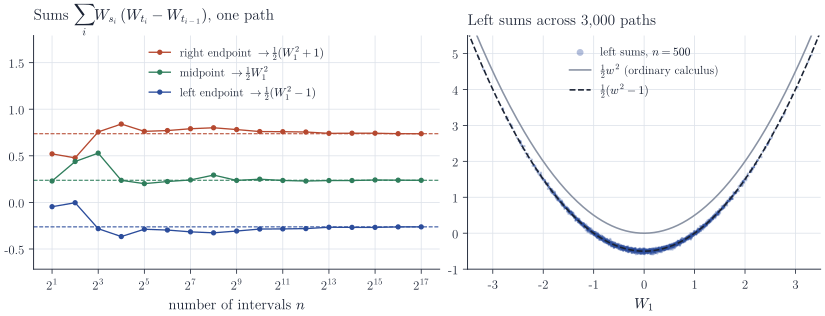
Itô’s choice of the left endpoint is not arbitrary. With \(H_{t_{i-1}}\) known at time \(t_{i-1}\) and \(\Delta_i W\) independent of \(\mathcal F_{t_{i-1}}\), each term has conditional mean zero, so Itô integrals are martingales. Indeed \(\tfrac12(W_t^2 - t)\) is a martingale, while \(\tfrac12W_t^2\) is not.
Itô’s formula for Brownian motion
Theorem 1 (Itô’s formula). Let \(f : \R \to \R\) be twice continuously differentiable with \(f'\) and \(f''\) bounded. Then for every \(t \ge 0\), almost surely,
\[f(W_t) = f(W_0) + \int_0^t f'(W_s)\,dW_s + \frac12\int_0^t f''(W_s)\,ds ,\]where the stochastic integral is the Itô integral of the bounded adapted process \(f'(W_s)\).
Proof. Fix \(t\) and partitions \(\pi\) with \(\abs{\pi} \to 0\). Telescoping and Taylor’s formula at \(W_{t_{i-1}}\) give the exact decomposition
\[f(W_t) - f(W_0) = \underbrace{\sum_i f'(W_{t_{i-1}})\,\Delta_i W}_{A_\pi} + \underbrace{\frac12\sum_i f''(W_{t_{i-1}})(\Delta_i W)^2}_{B_\pi} + \underbrace{\sum_i R_i}_{C_\pi},\]where \(R_i\) is defined by this identity term by term. We show that \(A_\pi\), \(B_\pi\) and \(C_\pi\) converge in probability to the two integrals and to zero. Let \(K\) bound \(\abs{f'}\) and \(\abs{f''}\).
The first-order term. \(A_\pi\) is the Itô integral of the simple process \(H^\pi_s = f'(W_{t_{i-1}})\) for \(s \in (t_{i-1}, t_i]\). By linearity and the isometry,
\[\E\Bigl(A_\pi - \int_0^t f'(W_s)\,dW_s\Bigr)^2 = \E\int_0^t \bigl(f'(W_s) - H^\pi_s\bigr)^2\,ds .\]The integrand is bounded by \(4K^2\) and tends to zero for every \((\omega, s)\) because \(f'\) and the paths are continuous. By dominated convergence on \(\Omega \times [0,t]\), \(A_\pi \to \int_0^t f'(W_s)\,dW_s\) in \(L^2\).
The second-order term. Write \(g_i = f''(W_{t_{i-1}})\), which is \(\mathcal F_{t_{i-1}}\)-measurable and bounded by \(K\), and split
\[2B_\pi = \sum_i g_i\,\Delta t_i + \sum_i g_i\bigl((\Delta_i W)^2 - \Delta t_i\bigr).\]The first sum is a Riemann sum of the continuous function \(s \mapsto f''(W_s)\) and converges pathwise to \(\int_0^t f''(W_s)\,ds\). In the second sum the terms are orthogonal: for \(i < j\), conditioning on \(\mathcal F_{t_{j-1}}\) and using \(\E[(\Delta_j W)^2 - \Delta t_j \mid \mathcal F_{t_{j-1}}] = 0\) shows that the cross products have mean zero. Hence
\[\E\Bigl(\sum_i g_i\bigl((\Delta_i W)^2 - \Delta t_i\bigr)\Bigr)^2 = \sum_i \E[g_i^2]\cdot 2(\Delta t_i)^2 \le 2K^2 t\,\abs{\pi} \to 0 .\]The remainder. By Taylor’s theorem with the Lagrange remainder, \(R_i = \tfrac12\bigl(f''(\eta_i) - f''(W_{t_{i-1}})\bigr)(\Delta_i W)^2\) for some \(\eta_i\) between \(W_{t_{i-1}}\) and \(W_{t_i}\), so
\[\abs{C_\pi} \le \frac12\,\max_i\,\omega_i \cdot \sum_i(\Delta_i W)^2, \qquad \omega_i = \sup\bigl\{\abs{f''(y) - f''(W_{t_{i-1}})} : \abs{y - W_{t_{i-1}}} \le \abs{\Delta_i W}\bigr\}.\]For fixed \(\omega\) the path on \([0,t]\) stays in a compact interval \(I\), \(f''\) is uniformly continuous on the 1-neighbourhood of \(I\), and \(\max_i\abs{\Delta_i W} \to 0\) by uniform continuity of the path; hence \(\max_i\omega_i \to 0\) pathwise. Since \(\sum_i(\Delta_i W)^2 \to t\) in probability, \(C_\pi \to 0\) in probability.
The left-hand side of the decomposition does not depend on \(\pi\), and limits in probability are unique up to null sets, which gives the formula.
Both sides of the formula are continuous in \(t\) (the stochastic integral has a continuous version), so the identity holds for all \(t\) simultaneously, outside a single null set. The boundedness of \(f'\) and \(f''\) is a convenience. For general \(f \in C^2\) one applies the theorem to a function that agrees with \(f\) on \([-R, R]\), stops the process when \(\abs{W}\) first reaches \(R\), and lets \(R \to \infty\); the stochastic integral is then understood in the extended sense, for integrands with \(\int_0^t H_s^2\,ds < \infty\) almost surely. With \(f(x) = x^2\) the formula returns \(W_t^2 = 2\int_0^t W_s\,dW_s + t\), as computed directly above.
The general form
The same argument, with \(\sum_i(\Delta_i X)^2 \to \int_0^t\sigma_s^2\,ds\) in place of \(\sum_i(\Delta_i W)^2 \to t\), handles Itô processes \(dX_t = \mu_t\,dt + \sigma_t\,dW_t\), with \(\mu\) and \(\sigma\) progressively measurable and \(\int_0^t (\abs{\mu_s} + \sigma_s^2)\,ds < \infty\) almost surely, and functions that also depend on time. For \(f(t, x)\) continuously differentiable in \(t\) and twice in \(x\),
\[\begin{equation} df(t, X_t) = \partial_t f(t, X_t)\,dt + \partial_x f(t, X_t)\,dX_t + \tfrac12\,\partial_{xx} f(t, X_t)\,\sigma_t^2\,dt . \label{eq:ito} \end{equation}\]A convenient bookkeeping device is to expand \(f\) to second order and apply the rules \((dt)^2 = 0\), \(dt\,dW_t = 0\), \((dW_t)^2 = dt\), so that \((dX_t)^2 = \sigma_t^2\,dt\). The rules summarize which sums of products of increments vanish in the limit and which converge to elapsed time.
Examples
Geometric Brownian motion. Consider \(dS_t = \mu S_t\,dt + \sigma S_t\,dW_t\) with \(S_0 > 0\). The coefficients are Lipschitz, so the equation has a unique solution, and we can verify a candidate. Let \(f(t, x) = S_0\exp\bigl((\mu - \tfrac12\sigma^2)t + \sigma x\bigr)\), so that \(\partial_t f = (\mu - \tfrac12\sigma^2)f\), \(\partial_x f = \sigma f\) and \(\partial_{xx}f = \sigma^2 f\). By \(\eqref{eq:ito}\) with \(X = W\),
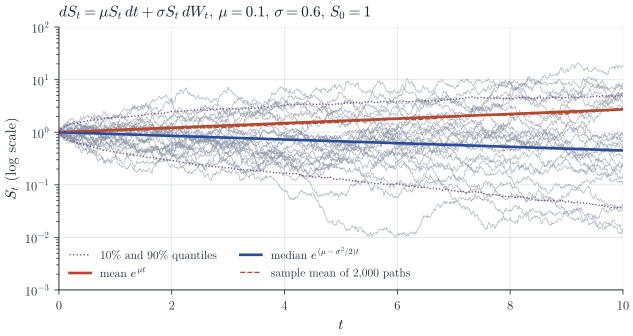
\[df(t, W_t) = \bigl(\mu - \tfrac12\sigma^2\bigr)f\,dt + \sigma f\,dW_t + \tfrac12\sigma^2 f\,dt = \mu f\,dt + \sigma f\,dW_t ,\]so \(S_t = S_0\exp\bigl((\mu - \tfrac12\sigma^2)t + \sigma W_t\bigr)\). The correction term changes the qualitative behaviour. Since \(\E e^{\sigma W_t} = e^{\sigma^2 t/2}\), the mean is \(\E S_t = S_0e^{\mu t}\). The median, however, is \(S_0e^{(\mu - \sigma^2/2)t}\), and since \(W_t/t \to 0\) almost surely,
\[\frac1t\log\frac{S_t}{S_0} = \mu - \frac{\sigma^2}{2} + \sigma\frac{W_t}{t} \longrightarrow \mu - \frac{\sigma^2}{2} \quad \text{almost surely}.\]If \(0 < \mu < \sigma^2/2\), the mean grows exponentially while almost every path tends to zero. Figure 2 shows this with \(\mu = 0.1\) and \(\sigma = 0.6\), where \(\mu - \sigma^2/2 = -0.08\): the mean is carried by a small fraction of paths with very large values.
The Ornstein–Uhlenbeck process. For \(dY_t = -\kappa Y_t\,dt + \sigma\,dW_t\) with \(\kappa > 0\), apply \(\eqref{eq:ito}\) to \(f(t, y) = e^{\kappa t}y\), for which \(\partial_{yy}f = 0\):
\[d\bigl(e^{\kappa t}Y_t\bigr) = \kappa e^{\kappa t}Y_t\,dt + e^{\kappa t}\bigl(-\kappa Y_t\,dt + \sigma\,dW_t\bigr) = \sigma e^{\kappa t}\,dW_t .\]Hence \(Y_t = e^{-\kappa t}Y_0 + \sigma\int_0^t e^{-\kappa(t-s)}\,dW_s\). For deterministic \(Y_0 = y_0\) the integral of a deterministic function is Gaussian (an \(L^2\) limit of Gaussian sums), with mean zero and, by the isometry, variance \(\sigma^2\int_0^t e^{-2\kappa(t-s)}\,ds = \sigma^2(1 - e^{-2\kappa t})/(2\kappa)\). So \(Y_t \sim N\bigl(y_0e^{-\kappa t}, \sigma^2(1 - e^{-2\kappa t})/(2\kappa)\bigr)\), which converges to the stationary law \(N(0, \sigma^2/(2\kappa))\) as \(t \to \infty\).
Exponential martingales. For \(\theta \in \R\) let \(Z_t = \exp(\theta W_t - \tfrac12\theta^2 t)\). Formula \(\eqref{eq:ito}\) gives \(dZ_t = \theta Z_t\,dW_t\), with no \(dt\) term. That \(Z\) is a genuine martingale, not only a stochastic integral, can be checked directly: for \(s < t\), \(\E[Z_t \mid \mathcal F_s] = Z_s\,\E\exp\bigl(\theta(W_t - W_s) - \tfrac12\theta^2(t-s)\bigr) = Z_s\). These processes are the densities in Girsanov’s change of measure.
Remarks
Stratonovich integrals, defined through midpoint evaluation, obey the ordinary chain rule, which makes them natural in physical modelling and on manifolds; the two calculi are related by the conversion \(\int_0^t H_s \circ dW_s = \int_0^t H_s\,dW_s + \tfrac12\langle H, W\rangle_t\), where \(H\) is a continuous semimartingale and \(\langle H, W\rangle\) is the quadratic covariation. Itô integrals are preferred in probability and finance because they produce martingales, as the computation of \(\int W\,dW\) already shows.
Complete treatments are in B. Øksendal, Stochastic Differential Equations; I. Karatzas and S. E. Shreve, Brownian Motion and Stochastic Calculus; and J. M. Steele, Stochastic Calculus and Financial Applications.