Sampling a posterior with a Markov chain: Metropolis–Hastings, Gibbs and what makes them work
A Bayesian analysis ends with a posterior density
\[\pi(\theta) = \pi(\theta \mid y) = \frac{p(y \mid \theta)\, p(\theta)}{\int p(y \mid \vartheta)\, p(\vartheta)\, \dd\vartheta},\]and almost every quantity of interest is an integral against it: posterior means and variances, tail probabilities, predictive densities. The numerator is usually available in closed form. The denominator, the marginal likelihood, is an integral over the whole parameter space and usually is not. Deterministic quadrature handles two or three dimensions, and importance sampling handles a few more if a good proposal is available, but both degrade quickly with dimension.
Markov chain Monte Carlo replaces independent draws by a dependent sequence \(\theta_0, \theta_1, \dots\) whose transition rule uses \(\pi\) only through ratios \(\pi(\theta')/\pi(\theta)\), so the normalizing constant cancels. The price is that the draws are correlated and only asymptotically distributed according to \(\pi\). Both the validity of the construction and the factors that govern its efficiency can be seen on one small model, used throughout.
A running example
Let \(y_1, \dots, y_n\) be independent \(N(\mu, 1/\tau)\) given the mean \(\mu\) and the precision \(\tau > 0\), with independent priors \(\mu \sim N(0, 1/\kappa_0)\) and \(\tau \sim \mathrm{Gamma}(a_0, b_0)\) (shape–rate). Writing \(S(\mu) = \sum_{i}(y_i - \mu)^2\), the posterior density on \(\R \times (0, \infty)\) is
\[\pi(\mu, \tau) \propto \tau^{a_0 + n/2 - 1} \exp\Bigl\{-\tau\bigl(b_0 + \tfrac12 S(\mu)\bigr) - \tfrac12 \kappa_0 \mu^2\Bigr\}.\]The prior is not conjugate for the pair, and the posterior is not a standard family. Its two full conditionals are standard, however. As a function of \(\tau\) alone the density is a Gamma kernel, and as a function of \(\mu\) alone the exponent is quadratic; completing the square gives
\[\tau \mid \mu, y \sim \mathrm{Gamma}\Bigl(a_0 + \frac n2,\; b_0 + \frac{S(\mu)}{2}\Bigr), \qquad \mu \mid \tau, y \sim N\Bigl(\frac{\tau \sum_i y_i}{n\tau + \kappa_0},\; \frac{1}{n\tau + \kappa_0}\Bigr).\]In the figures, \(n = 12\) observations are simulated from \(N(1.5, 0.8^2)\), and \(\kappa_0 = 10^{-2}\), \(a_0 = 2\), \(b_0 = 1\). The problem is two-dimensional, so quadrature would also do; it is small enough to draw.
Invariance and detailed balance
Let \((E, \mathcal E)\) be the state space, here a subset of \(\R^d\) with its Borel sets, and \(P(x, A)\) a Markov kernel: a probability measure in \(A\) for each \(x\), and measurable in \(x\) for each \(A\). A probability measure \(\pi\) is invariant for \(P\) if
\[\pi P(A) := \int_E \pi(\dd x)\, P(x, A) = \pi(A) \qquad \text{for all } A \in \mathcal E,\]so that \(X_0 \sim \pi\) implies \(X_t \sim \pi\) for every \(t\). The kernel is reversible with respect to \(\pi\) if the joint law of \((X_0, X_1)\) is symmetric when \(X_0 \sim \pi\):
\[\int_A \pi(\dd x)\, P(x, B) = \int_B \pi(\dd x)\, P(x, A) \qquad \text{for all } A, B \in \mathcal E.\]Taking \(A = E\) gives \(\pi P(B) = \int_B \pi(\dd x) P(x, E) = \pi(B)\), so reversibility implies invariance. It is the condition that MCMC constructions check, because it can be verified pair of states by pair of states, without computing any integral.
The Metropolis–Hastings kernel
Suppose \(\pi\) has a density, also written \(\pi\), with respect to a reference measure \(\lambda\) (Lebesgue measure in the example), and let \(q(x, y)\) be a proposal density: \(y \mapsto q(x, y)\) is a probability density for each \(x\). From the current state \(x\), draw \(Y \sim q(x, \cdot)\) and move to \(Y\) with probability \(\alpha(x, Y)\), otherwise stay at \(x\), where
\[\alpha(x, y) = \begin{cases} \min\Bigl\{1, \dfrac{\pi(y)\, q(y, x)}{\pi(x)\, q(x, y)}\Bigr\}, & \pi(x) q(x, y) > 0,\\[1ex] 1, & \text{otherwise.} \end{cases}\]Only the ratio \(\pi(y)/\pi(x)\) enters, so \(\pi\) may be specified up to a constant. The resulting kernel is
\[P(x, \dd y) = q(x, y)\, \alpha(x, y)\, \lambda(\dd y) + r(x)\, \delta_x(\dd y), \qquad r(x) = 1 - \int_E q(x, z)\, \alpha(x, z)\, \lambda(\dd z),\]with \(r(x)\) the probability of rejection.
Proposition 1. The Metropolis–Hastings kernel is reversible with respect to \(\pi\); in particular \(\pi\) is invariant.
Proof. The definition of \(\alpha\) gives, for all \(x, y\),
\[\pi(x)\, q(x, y)\, \alpha(x, y) = \min\bigl\{\pi(x) q(x, y),\; \pi(y) q(y, x)\bigr\}.\]When \(\pi(x) q(x, y) > 0\) this is the identity \(a \min\{1, b/a\} = \min\{a, b\}\); when \(\pi(x) q(x, y) = 0\) both sides vanish. The right-hand side is symmetric in \((x, y)\). Hence for \(A, B \in \mathcal E\)
\[\int_A \pi(\dd x) P(x, B) = \int_A \int_B \min\bigl\{\pi(x) q(x, y), \pi(y) q(y, x)\bigr\}\, \lambda(\dd y)\, \lambda(\dd x) + \int_{A \cap B} r(x)\, \pi(x)\, \lambda(\dd x),\]and both terms are unchanged when \(A\) and \(B\) are exchanged (Tonelli’s theorem allows the order of integration in the first term to be swapped, since the integrand is nonnegative).
The random-walk Metropolis algorithm takes \(q(x, y) = h^{-d} \phi\bigl((y - x)/h\bigr)\) with \(\phi\) the standard normal density in \(\R^d\) and a scale \(h > 0\). The proposal is symmetric, so \(\alpha(x, y) = \min\{1, \pi(y)/\pi(x)\}\): moves uphill are always accepted and moves downhill are accepted with probability equal to the density ratio.
A random walk on \(\R^d\) needs the target on \(\R^d\), so in the example we sample \((\mu, \eta)\) with \(\eta = \log \tau\). The change of variables \(\tau = e^\eta\) has Jacobian \(e^\eta\), and the target becomes
\[\log \pi(\mu, \eta) = \Bigl(a_0 + \frac n2\Bigr) \eta - e^{\eta}\Bigl(b_0 + \frac{S(\mu)}{2}\Bigr) - \frac{\kappa_0 \mu^2}{2} + \text{const}.\]Omitting the Jacobian is a common error. The chain would still converge, but to the wrong distribution, one whose \(\tau\)-marginal is proportional to \(\tau^{-1}\) times the correct one.
The Gibbs sampler
Write \(x = (x_1, x_2)\) with blocks \(x_1 \in E_1\), \(x_2 \in E_2\), and let \(\pi(\dd x_1 \mid x_2)\) be a regular conditional distribution of the first block given the second under \(\pi\). The Gibbs kernel for the first block resamples it from its conditional and leaves the second block fixed:
\[K_1\bigl((x_1, x_2), A\bigr) = \int_{E_1} \mathbf 1_A(z, x_2)\, \pi(\dd z \mid x_2).\]Proposition 2. \(K_1\) is reversible with respect to \(\pi\). Consequently the systematic-scan Gibbs sampler \(K_1 K_2\), which updates the two blocks in turn, has \(\pi\) as an invariant distribution.
Proof. Let \(X = (X_1, X_2) \sim \pi\) and, conditionally on \(X\), draw \(Z \sim \pi(\cdot \mid X_2)\). Then \((X, (Z, X_2))\) has the law \(\pi(\dd x) K_1(x, \dd x')\). Given \(X_2\), the variables \(X_1\) and \(Z\) are independent with the same law \(\pi(\cdot \mid X_2)\), so the pair \(\bigl((X_1, X_2), (Z, X_2)\bigr)\) has the same distribution as \(\bigl((Z, X_2), (X_1, X_2)\bigr)\). This exchangeability is reversibility. Since both \(K_1\) and \(K_2\) leave \(\pi\) invariant, \(\pi K_1 K_2 = \pi K_2 = \pi\).
The composition \(K_1 K_2\) is in general not reversible, which matters for parts of the central limit theory below but not for invariance. Equivalently, \(K_1\) is the Metropolis–Hastings kernel with proposal \(\pi(\cdot \mid x_2)\) for the first block; substituting into the acceptance ratio shows that every proposal is accepted.
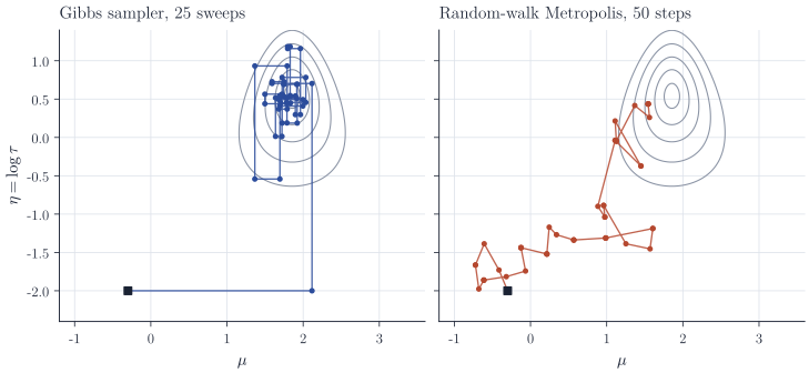
Figure 1 shows the two samplers started at the same point far in the tail. Gibbs moves parallel to the coordinate axes, and here reaches the bulk of the posterior in a single sweep because each conditional is sampled exactly. Random-walk Metropolis approaches by small steps and stays where it is whenever a proposal is rejected.
Why ergodic averages converge
Invariance says that a chain started from \(\pi\) stays at \(\pi\). It says nothing about a chain started elsewhere, and it does not rule out chains that never leave a region: the kernel \(P(x, \cdot) = \delta_x\) leaves every distribution invariant. The missing ingredient is irreducibility. A kernel is \(\pi\)-irreducible if from every starting point it reaches every set of positive \(\pi\)-measure with positive probability in some number of steps.
For random-walk Metropolis on a target with an everywhere positive density, as in the example, irreducibility holds after one step: if \(\pi(A) > 0\) then \(P(x, A) \ge \int_A q(x, y) \alpha(x, y)\, \dd y > 0\), because the integrand is positive on \(A\). Tierney (1994) shows that a \(\pi\)-irreducible Metropolis–Hastings kernel is also Harris recurrent. For a Harris recurrent chain with invariant distribution \(\pi\) and every \(h \in L^1(\pi)\), the ergodic theorem gives
\[\bar h_T = \frac1T \sum_{t=1}^T h(X_t) \xrightarrow{\text{a.s.}} \int h \, \dd \pi \qquad (T \to \infty)\]from every initial state. Aperiodicity is not needed for this law of large numbers. It is needed for the stronger statement that the law of \(X_t\) converges to \(\pi\) in total variation from every starting point; random-walk Metropolis on an everywhere positive density is aperiodic, since \(P(x, A) > 0\) for every \(x\) and every \(A\) of positive Lebesgue measure. This convergence in law is what makes the common practice of discarding an initial segment (burn-in) reasonable: after enough iterations the draws are approximately distributed according to \(\pi\).
Efficiency and the proposal scale
All valid samplers have the same limit; they differ in how fast \(\bar h_T\) gets there. When a central limit theorem holds, \(\sqrt T(\bar h_T - \pi h) \Rightarrow N(0, \sigma_h^2)\) with
\[\sigma_h^2 = \Var_\pi\bigl(h(X_0)\bigr)\Bigl(1 + 2 \sum_{k \ge 1} \rho_k\Bigr), \qquad \rho_k = \Corr_\pi\bigl(h(X_0), h(X_k)\bigr),\]the correlations computed for the stationary chain and the series assumed convergent. For a reversible chain started in stationarity and \(h \in L^2(\pi)\), the central limit theorem holds whenever \(\lim_{T} T \Var(\bar h_T) < \infty\), by a theorem of Kipnis and Varadhan (1986). Without reversibility, a sufficient condition is geometric ergodicity together with \(\E_\pi \abs{h}^{2+\delta} < \infty\) for some \(\delta > 0\). For a Harris recurrent chain, a central limit theorem that holds under stationarity holds for every initial distribution, so the burn-in does not affect the limit. The ratio \(T \Var_\pi(h)/\sigma_h^2\) is the effective sample size: the number of independent draws that would give the same Monte Carlo variance.
For random-walk Metropolis the scale \(h\) controls the autocorrelations directly. Small \(h\) gives proposals close to the current state, which are almost always accepted but move the chain very little. Large \(h\) gives proposals that mostly land in the tails and are rejected, so the chain stands still for long stretches. In both cases \(\rho_k\) decays slowly and \(\sigma_h^2\) is large. Figure 2 shows the three regimes on the running example.
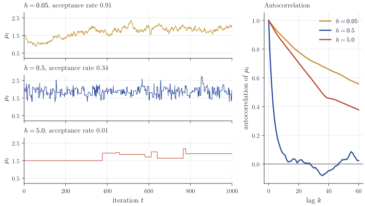
There is a theory for the intermediate choice. For targets that are products of \(d\) identical one-dimensional densities and Gaussian random-walk proposals with scale proportional to \(d^{-1/2}\), Roberts, Gelman and Gilks (1997) show that, as \(d \to \infty\), the efficiency is maximized when the acceptance rate is about \(0.234\). The result is asymptotic and for a special class of targets, but acceptance rates between roughly \(0.2\) and \(0.5\) are a sensible default in moderate dimension, and adaptive schemes tune \(h\) toward them during burn-in.
Remarks
The example illustrates the two basic strategies. Gibbs sampling exploits conditional structure and needs no tuning, but it moves only along coordinate directions, so it slows down when the parameters are strongly correlated a posteriori. Random-walk Metropolis needs only pointwise evaluation of \(\log\pi\), but its steps must shrink as the dimension grows. Gradient-based proposals such as Hamiltonian Monte Carlo and auxiliary-variable methods such as slice sampling address these weaknesses within the same framework: each constructs a kernel that is reversible, or at least invariant, with respect to \(\pi\).
Standard references are Robert and Casella, Monte Carlo Statistical Methods, for the algorithms, and Meyn and Tweedie, Markov Chains and Stochastic Stability, for the general state-space theory. The convergence results for Metropolis–Hastings used above are in Tierney, “Markov chains for exploring posterior distributions” (Annals of Statistics, 1994), and Roberts and Rosenthal, “General state space Markov chains and MCMC algorithms” (Probability Surveys, 2004).