Fair games and when to stop them: martingales and the optional stopping theorem

A gambler playing a fair game cannot expect to win, whatever the stakes on each round and whenever the gambler decides to leave the table, provided the decisions use only past outcomes and the gambler cannot play forever. Martingales are the mathematical form of a fair game, and this statement, made precise, is the optional stopping theorem. The qualifier at the end matters: there are stopping rules that guarantee a profit if one can wait indefinitely, and the way they fail explains the conditions of the theorem.

Throughout, $(\Omega, \mathcal F, \P)$ is a probability space with a filtration $\mathcal F_0 \subseteq \mathcal F_1 \subseteq \cdots \subseteq \mathcal F$; $\mathcal F_n$ is the information available at time $n$.

Definition and examples

A sequence $(M_n)_{n\ge0}$ is a martingale if each $M_n$ is $\mathcal F_n$-measurable and integrable and

\[\E[M_{n+1} \mid \mathcal F_n] = M_n \quad \text{almost surely, for all } n \ge 0 .\]

With $\le$ in place of $=$ it is a supermartingale (an unfavourable game), with $\ge$ a submartingale. Equivalently, the increments $D_n = M_n - M_{n-1}$ satisfy $\E[D_n \mid \mathcal F_{n-1}] = 0$: given the past, the next increment is unpredictable in mean. If the $M_n$ are square integrable, the increments are orthogonal, since for $m < n$, $\E[D_mD_n] = \E[D_m\E(D_n \mid \mathcal F_{n-1})] = 0$, and hence $\E M_n^2 = \E M_0^2 + \sum_{k=1}^n\E D_k^2$.

Some examples that recur below:

Random walks. If $\xi_1, \xi_2, \dots$ are independent with mean zero and $\mathcal F_n = \sigma(\xi_1, \dots, \xi_n)$, then $S_n = \xi_1 + \dots + \xi_n$ is a martingale. If moreover $\Var\xi_i = 1$, so is $S_n^2 - n$, because $\E[S_{n+1}^2 - S_n^2 \mid \mathcal F_n] = 2S_n\E\xi_{n+1} + \E\xi_{n+1}^2 = 1$.
Products. If the $\xi_i$ are independent, nonnegative and have mean one, $\prod_{i\le n}\xi_i$ is a martingale. For a simple random walk with $\P(\xi_i = 1) = p$, $\P(\xi_i = -1) = q = 1 - p$, the choice $(q/p)^{\xi_i}$ gives the martingale $(q/p)^{S_n}$.
Likelihood ratios. Let $X_1, X_2, \dots$ be independent with density $p$, and let $q$ be another density. Then $L_n = \prod_{i\le n}q(X_i)/p(X_i)$ is a product of nonnegative factors with $\E[q(X_i)/p(X_i)] = \int_{\{p > 0\}}q \le 1$, hence a nonnegative supermartingale, and a martingale when $q = 0$ wherever $p = 0$.
Accumulating information. For an integrable $Y$, $M_n = \E[Y \mid \mathcal F_n]$ is a martingale by the tower property: the sequence of best predictions of $Y$ as information grows.

Betting systems and stopping times

A process $(H_n)_{n\ge1}$ is predictable if $H_n$ is $\mathcal F_{n-1}$-measurable: the stake on round $n$ is chosen before the round is played. The gambler’s accumulated gain is the martingale transform

\[(H \cdot M)_n = \sum_{k=1}^n H_k(M_k - M_{k-1}) .\]

Proposition 1. Let $H$ be predictable and bounded. If $M$ is a martingale, so is $(H\cdot M)$. If $M$ is a supermartingale and $H \ge 0$, then $(H\cdot M)$ is a supermartingale.

Proof. $(H\cdot M)_n$ is $\mathcal F_n$-measurable and integrable because $H$ is bounded. Since $H_{n+1}$ is $\mathcal F_n$-measurable, $\E[(H\cdot M)_{n+1} - (H\cdot M)_n \mid \mathcal F_n] = H_{n+1}\E[M_{n+1} - M_n \mid \mathcal F_n]$, which is zero in the first case and nonpositive in the second.

A stopping time is a random variable $\tau$ with values in $\{0, 1, 2, \dots\} \cup \{\infty\}$ such that $\{\tau \le n\} \in \mathcal F_n$ for every $n$: whether to stop by time $n$ is decided by the information at time $n$. Playing one unit until $\tau$ means $H_k = \mathbf 1\{\tau \ge k\}$, which is predictable because $\{\tau \ge k\} = \{\tau \le k-1\}^c \in \mathcal F_{k-1}$. The resulting transform is $(H\cdot M)_n = M_{\tau\wedge n} - M_0$. By Proposition 1 the stopped process $(M_{\tau\wedge n})_{n\ge0}$ is a martingale (a supermartingale) whenever $M$ is, and in particular

\[\begin{equation} \E M_{\tau\wedge n} = \E M_0 \quad (\text{martingale}), \qquad \E M_{\tau\wedge n} \le \E M_0 \quad (\text{supermartingale}), \qquad n \ge 0 . \label{eq:stopped} \end{equation}\]

Optional stopping

The question is when $\eqref{eq:stopped}$ survives the limit $n \to \infty$, so that $\E M_\tau = \E M_0$.

Theorem 2 (Optional stopping). Let $M$ be a martingale and $\tau$ a stopping time. Each of the following conditions implies that $M_\tau$ is integrable and $\E M_\tau = \E M_0$:

$\tau \le N$ almost surely for some constant $N$;
$\tau < \infty$ almost surely and $\abs{M_{\tau\wedge n}} \le K$ for all $n$, for some constant $K$;
$\E\tau < \infty$ and $\abs{M_n - M_{n-1}} \le c$ for all $n$, for some constant $c$.

Proof. Under condition 1, take $n = N$ in $\eqref{eq:stopped}$. Under conditions 2 and 3, $\tau < \infty$ almost surely, so $M_{\tau\wedge n} \to M_\tau$ almost surely, and it suffices to dominate $\abs{M_{\tau\wedge n}}$ by an integrable variable and apply dominated convergence to $\eqref{eq:stopped}$. Under condition 2 the constant $K$ serves. Under condition 3,

\[\abs{M_{\tau\wedge n}} \le \abs{M_0} + \sum_{k=1}^{\tau\wedge n}\abs{M_k - M_{k-1}} \le \abs{M_0} + c\,\tau,\]

which is integrable.

Some condition of this kind is necessary. Let $S_n$ be a simple symmetric random walk started at $0$ and $\tau = \min\{n : S_n = 1\}$. The walk is recurrent, so $\tau < \infty$ almost surely, and $S_\tau = 1$, so $\E S_\tau = 1 \ne 0 = \E S_0$. “Play until you are one unit ahead” is a winning strategy, provided one has unlimited time and credit. Here $\E\tau = \infty$, and $S_{\tau\wedge n}$ is unbounded below, so neither condition 2 nor condition 3 holds. Before the stopping time, the walk can wander arbitrarily far into losses, and the guaranteed final gain is financed by these losses on paths that take very long.

The gambler’s ruin

Let $S_n$ be a simple symmetric random walk from $0$, let $a, b$ be positive integers, and let $\tau$ be the first time $S$ reaches $-a$ or $b$.

First, $\E\tau < \infty$. In any block of $a + b$ consecutive steps, if all steps are $+1$ the walk must leave $(-a, b)$; this event has probability $2^{-(a+b)}$ and the blocks are independent, so $\P(\tau > j(a+b)) \le (1 - 2^{-(a+b)})^j$, a geometric tail.

Exit probabilities. The increments of $S$ are bounded by one, so condition 3 of Theorem 2 applies: $0 = \E S_\tau = b\,\P(S_\tau = b) - a\,(1 - \P(S_\tau = b))$, and

\[\P(S_\tau = b) = \frac{a}{a + b} .\]

Expected duration. The martingale $S_n^2 - n$ does not have bounded increments, but $\eqref{eq:stopped}$ gives $\E S_{\tau\wedge n}^2 = \E(\tau\wedge n)$ for each $n$. As $n \to \infty$ the left side converges to $\E S_\tau^2$ by bounded convergence ($\abs{S_{\tau\wedge n}} \le \max(a, b)$) and the right side to $\E\tau$ by monotone convergence. Hence

\[\E\tau = \E S_\tau^2 = b^2\frac{a}{a+b} + a^2\frac{b}{a+b} = ab .\]

For a biased walk with $p \ne q$, the block argument (now with probability $p^{a+b}$ for a run of upward steps) again gives $\tau < \infty$ almost surely, and the stopped martingale $r^{S_{\tau\wedge n}}$, $r = q/p$, is bounded by $\max(r^b, r^{-a})$. Bounded convergence in $\eqref{eq:stopped}$ gives $1 = r^b\,\P(S_\tau = b) + r^{-a}(1 - \P(S_\tau = b))$, so $\P(S_\tau = b) = (1 - r^{-a})/(r^b - r^{-a})$.

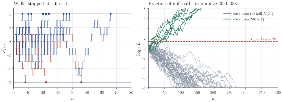
With $a = 6$ and $b = 4$, the walk exits at the top with probability $0.6$ after $24$ steps on average. The left panel of Figure 1 shows stopped paths; in $10^5$ simulated walks the proportion exiting at the top was $0.600$ and the mean exit time $24.1$.

Random walk paths stopped at two barriers, and likelihood ratio martingale paths under null and alternative with a horizontal threshold at twenty — Figure 1. Left: fourteen simple random walks from $0$, stopped on reaching $4$ (blue) or $-6$ (red). Right: $\log_{10}$ of the likelihood ratio $L_n$ of $N(0.5, 1)$ against $N(0,1)$, for 40 sequences generated under the null (grey) and 8 under the alternative (green). In $2 \times 10^4$ null sequences of length 400, a fraction $0.038$ ever reached $L_n \ge 20$, below the bound $\alpha = 0.05$ of Ville's inequality.

Ville’s inequality and tests that may be stopped at any time

Optional stopping also controls the whole path of a nonnegative supermartingale.

Proposition 3 (Ville’s inequality). If $(M_n)$ is a nonnegative supermartingale, then $\P\bigl(\sup_{n\ge0}M_n \ge c\bigr) \le \E M_0/c$ for every $c > 0$.

Proof. Let $\tau = \min\{n : M_n \ge c\}$, a stopping time. For each $n$, by $\eqref{eq:stopped}$ and nonnegativity,

\[\E M_0 \ge \E M_{\tau\wedge n} \ge \E\bigl[M_\tau\mathbf 1\{\tau \le n\}\bigr] \ge c\,\P(\tau \le n).\]

Letting $n \to \infty$ gives $\P(\tau < \infty) \le \E M_0/c$, and $\{\tau < \infty\} = \{\sup_n M_n \ge c\}$.

Applied to the likelihood ratio of example 3, which has $L_0 = 1$, this yields a test of the null hypothesis that the data have density $p$ against the alternative $q$: reject as soon as $L_n \ge 1/\alpha$. Under the null,

\[\P_p\bigl(L_n \ge 1/\alpha \text{ for some } n\bigr) \le \alpha,\]

so the type I error is controlled uniformly over time. The analyst may look at the data after every observation, stop for any reason, or continue indefinitely, and the guarantee holds. Repeating a fixed-sample-size test at level $\alpha$ after each observation behaves very differently: for the one-sided $z$-test that rejects when $S_n/\sqrt n$ exceeds a fixed quantile, the law of the iterated logarithm implies that under the null the statistic exceeds every fixed level infinitely often, so the probability of a false rejection at some time is one.

For the Gaussian example in Figure 1, with $p = N(0,1)$ and $q = N(\theta, 1)$, $\log L_n = \theta S_n - n\theta^2/2$ where $S_n = X_1 + \dots + X_n$. Under the null $S_n/n \to 0$ almost surely, so $\log L_n \to -\infty$ and $L_n \to 0$ almost surely, even though $\E L_n = 1$ for every $n$. The mean is carried by rare paths with large values, the same phenomenon as in the walk that stops at $+1$; here it is harmless, because Ville’s inequality only needs the supermartingale inequality $\eqref{eq:stopped}$ at bounded times. Under the alternative, $\log L_n/n \to \theta^2/2 > 0$ almost surely, so the threshold is eventually crossed with probability one.

Remarks

Two further results complete the basic theory: Doob’s convergence theorem, which says that a martingale bounded in $L^1$ converges almost surely (so nonnegative martingales always converge, as the likelihood ratio did), and the optional stopping theorem for uniformly integrable martingales, which gives $\E M_\tau = \E M_0$ for every stopping time $\tau$, with $M_\tau$ defined on $\{\tau = \infty\}$ as the almost sure limit of $M_n$. Both are proved in D. Williams, Probability with Martingales, which is the natural next step; R. Durrett, Probability: Theory and Examples, covers the same ground.

The sequential likelihood ratio test above is closely related to A. Wald’s sequential probability ratio test. The modern theory of tests and confidence sequences that remain valid under optional stopping, built on nonnegative supermartingales and Ville’s inequality, is surveyed in A. Ramdas, P. Grünwald, V. Vovk and G. Shafer, “Game-theoretic statistics and safe anytime-valid inference” (Statistical Science, 2023).