One convex program seen from two sides: maximum entropy and maximum likelihood

Fitting an exponential family by maximum likelihood amounts to matching moments: the score equation says that the fitted model must reproduce the sample averages of the sufficient statistics. A different principle leads to the same place. Among all distributions whose moments equal those sample averages, choose the one of largest entropy. The two answers coincide, and the reason is that the two optimization problems are Lagrange duals of each other. The log-likelihood is, up to sign, the dual function of the entropy program.

The argument below is carried out on a finite sample space, where all quantities are finite sums and no regularity conditions are hidden. The continuous case is discussed at the end.

Setting

Let $\mathcal X$ be a finite set, $\Delta$ the set of probability vectors on $\mathcal X$, and $T : \mathcal X \to \R^k$ a statistic. Write $H(p) = -\sum_x p(x)\log p(x)$ for the entropy (with $0\log 0 = 0$), $\E_p T = \sum_x p(x)T(x)$, and

\[p_\theta(x) = \exp\bigl(\theta^\top T(x) - A(\theta)\bigr), \qquad A(\theta) = \log\sum_{x\in\mathcal X} e^{\theta^\top T(x)}, \qquad \theta \in \R^k,\]

for the exponential family generated by $T$. Given observations $x_1, \dots, x_n \in \mathcal X$ with empirical distribution $\hat p_n$, set $\hat t = \E_{\hat p_n} T = n^{-1}\sum_i T(x_i)$. The average log-likelihood is

\[\ell_n(\theta) = \frac1n\sum_{i=1}^n \log p_\theta(x_i) = \theta^\top \hat t - A(\theta),\]

which depends on the data only through $\hat t$. The two problems are

\[\text{(P)}\quad \max_{p\in\Delta} H(p) \ \text{ subject to } \ \E_p T = \hat t, \qquad\qquad \text{(D)}\quad \max_{\theta\in\R^k} \ell_n(\theta).\]

Problem (P) is feasible, since $\hat p_n$ satisfies its constraint. Its feasible set is compact and $H$ is continuous, so (P) always has a solution. Whether (D) has one is a separate question.

Two derivatives will be needed. Since $A$ is a logarithm of a finite sum of exponentials, it is infinitely differentiable, and direct computation gives

\[\nabla A(\theta) = \E_{\theta} T, \qquad \nabla^2 A(\theta) = \Cov_{\theta}(T),\]

where the subscript $\theta$ refers to $p_\theta$. In particular $A$ is convex, $\ell_n$ is concave, and $\nabla\ell_n(\theta) = \hat t - \E_\theta T$.

One identity

Lemma 1 (Gibbs variational identity). For every $p \in \Delta$ and $\theta \in \R^k$,

\[H(p) + \theta^\top \E_p T = A(\theta) - \KL(p\,\Vert\,p_\theta).\]

Consequently $\max_{p\in\Delta}\{H(p) + \theta^\top\E_p T\} = A(\theta)$, and $p_\theta$ is the unique maximizer.

Proof. Since $p_\theta(x) > 0$ for every $x$, the divergence is a finite sum:

\[\KL(p\,\Vert\,p_\theta) = \sum_x p(x)\log p(x) - \sum_x p(x)\bigl(\theta^\top T(x) - A(\theta)\bigr) = -H(p) - \theta^\top\E_p T + A(\theta).\]

The second statement follows because $\KL(p\,\Vert\,p_\theta) \ge 0$, with equality only when $p = p_\theta$ (Gibbs’ inequality).

In the language of convex analysis, Lemma 1 says that the log-partition function $A$ is the convex conjugate of the function $m \mapsto -\max\{H(p) : \E_p T = m\}$, since $\sup_m\{\theta^\top m + \max\{H(p) : \E_pT = m\}\} = \max_p\{H(p) + \theta^\top\E_pT\}$. Everything below is a consequence of the identity.

The dual function is the negative log-likelihood

Attach a multiplier $\theta \in \R^k$ to the constraint of (P) and form the Lagrangian

\[L(p, \theta) = H(p) + \theta^\top\bigl(\E_p T - \hat t\bigr), \qquad p \in \Delta .\]

The normalization $\sum_x p(x) = 1$ and the positivity constraints are kept in the domain $\Delta$ rather than dualized. By Lemma 1 the dual function is

\[g(\theta) = \max_{p\in\Delta} L(p, \theta) = A(\theta) - \theta^\top\hat t = -\ell_n(\theta),\]

and the maximizing $p$ is $p_\theta$. Minimizing the dual function is therefore exactly maximum likelihood in the family $p_\theta$. The exponential family appears here without having been postulated: it is the set of maximizers of the Lagrangian.

Weak duality takes a particularly sharp form. For $p$ feasible for (P), $\E_p T = \hat t$, and Lemma 1 rearranges to

\[\begin{equation} H(p) + \KL(p\,\Vert\,p_\theta) = -\ell_n(\theta) \qquad \text{for every feasible } p \text{ and every } \theta \in \R^k . \label{eq:pyth} \end{equation}\]

So $H(p) \le -\ell_n(\theta)$ for every feasible $p$ and every $\theta$, and the duality gap at the pair $(p, \theta)$ is exactly $\KL(p\,\Vert\,p_\theta)$. Taking $p = \hat p_n$ in $\eqref{eq:pyth}$ recovers a familiar fact: $-\ell_n(\theta)$ is the cross-entropy of $p_\theta$ relative to $\hat p_n$, and maximizing the likelihood is the same as minimizing $\KL(\hat p_n\,\Vert\,p_\theta)$ over $\theta$.

Strong duality when the maximum likelihood estimate exists

Theorem 2. For $\hat\theta \in \R^k$ the following are equivalent:

$\hat\theta$ maximizes $\ell_n$;
$\E_{\hat\theta} T = \hat t$;
$p_{\hat\theta}$ is feasible for (P).

If they hold, $p_{\hat\theta}$ is the unique solution of (P), and $\max\text{(P)} = H(p_{\hat\theta}) = -\ell_n(\hat\theta) = -\max\text{(D)}$.

Proof. A differentiable concave function on $\R^k$ is maximized exactly at its stationary points, and $\nabla\ell_n(\hat\theta) = \hat t - \E_{\hat\theta}T$; this gives the equivalence of 1 and 2. Statements 2 and 3 are the same by definition. Now apply $\eqref{eq:pyth}$ with $\theta = \hat\theta$. For $p = p_{\hat\theta}$, which is feasible, the divergence vanishes and $H(p_{\hat\theta}) = -\ell_n(\hat\theta)$. For any other feasible $p$ the divergence is positive, so $H(p) < H(p_{\hat\theta})$.

The proof yields two exact identities. Applying $\eqref{eq:pyth}$ to $p = p_{\hat\theta}$ and an arbitrary $\theta$ gives

\[\ell_n(\hat\theta) - \ell_n(\theta) = \KL(p_{\hat\theta}\,\Vert\,p_\theta),\]

so the log-likelihood ratio between the maximum likelihood fit and any other member of the family is a Kullback–Leibler divergence. Applying it to $p = \hat p_n$ at $\theta$ and at $\hat\theta$ and subtracting gives

\[\KL(\hat p_n\,\Vert\,p_\theta) = \KL(\hat p_n\,\Vert\,p_{\hat\theta}) + \KL(p_{\hat\theta}\,\Vert\,p_\theta),\]

a Pythagorean relation: $p_{\hat\theta}$ is the projection of $\hat p_n$ onto the exponential family in the Kullback–Leibler sense, and it lies on the set of distributions that share the moments of $\hat p_n$.

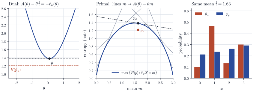
Figure 1 illustrates the picture with $\mathcal X = \{0, 1, 2, 3\}$, $T(x) = x$, and thirty simulated observations with $\hat t = 1.63$. The left panel is the dual objective. The middle panel shows the primal value $m \mapsto \max\{H(p) : \E_p X = m\}$ as the lower envelope of the lines $m \mapsto A(\theta) - \theta m$, one for each $\theta$; this is $\eqref{eq:pyth}$ read geometrically, and the line for $\hat\theta$ touches the envelope at $m = \hat t$. The empirical distribution has the same mean as $p_{\hat\theta}$ but entropy $1.216$ instead of $1.379$, the difference being $\KL(\hat p_n\,\Vert\,p_{\hat\theta}) \approx 0.163$.

Dual objective as a function of theta, the maximum entropy curve as a lower envelope of lines, and empirical versus fitted probabilities — Figure 1. Maximum entropy and maximum likelihood on $\{0,1,2,3\}$ with $T(x) = x$ and $n = 30$. Left: the dual function $A(\theta) - \theta\hat t$, minimized at the maximum likelihood estimate $\hat\theta$; its minimum value equals $H(p_{\hat\theta})$ and lies above $H(\hat p_n)$. Middle: the maximum entropy value as a function of the mean (blue) is the lower envelope of the lines $m \mapsto A(\theta) - \theta m$ (grey); the dashed line corresponds to $\hat\theta$. Right: the empirical distribution and the fitted $p_{\hat\theta}$, which have the same mean.

When the maximum likelihood estimate does not exist

Because $p_\theta$ charges every point of $\mathcal X$, the mean $\E_\theta T$ is a convex combination of all the points $T(x)$ with strictly positive weights, and so lies in the relative interior of the convex hull of $T(\mathcal X)$. If $\hat t$ lies on the relative boundary, no $\hat\theta$ satisfies condition 2 of Theorem 2, and (D) has no maximizer even though (P) has a solution. Conversely, if $\hat t$ lies in the relative interior, a maximizer exists; when $T$ is minimal (no nonzero $a$ makes $a^\top T$ constant on $\mathcal X$) the Hessian $\Cov_\theta(T)$ is positive definite and the maximizer is unique. Without minimality the maximizers form an affine subspace of $\R^k$, but they all define the same distribution $p_{\hat\theta}$, the unique solution of (P). This existence criterion is classical; see O. Barndorff-Nielsen, Information and Exponential Families in Statistical Theory.

In the example of Figure 1, suppose all observations equal $0$. Then $\hat t = 0$, the only feasible $p$ in (P) is the point mass at $0$, and $\max\text{(P)} = 0$. On the dual side, $\ell_n(\theta) = -\log(1 + e^\theta + e^{2\theta} + e^{3\theta})$ is negative for every $\theta$ and increases to $0$ as $\theta \to -\infty$. The optimal values still agree, but the dual optimum is approached only along a sequence that leaves every compact set, and the corresponding $p_\theta$ converge to the point mass. The same phenomenon is familiar from logistic regression with separable data, which is a conditional version of this problem.

Remarks

Two practical consequences follow from the duality. First, the dual has $k$ unconstrained variables while the primal has $\abs{\mathcal X}$ constrained ones, so maximum entropy problems with a large sample space are solved in the dual, for example by Newton’s method $\theta \leftarrow \theta + \Cov_\theta(T)^{-1}(\hat t - \E_\theta T)$, or by iterative scaling (J. N. Darroch and D. Ratcliff, “Generalized iterative scaling for log-linear models”, Annals of Mathematical Statistics, 1972). Second, multinomial logistic regression is the dual of a conditional maximum entropy problem, a connection exploited in A. L. Berger, S. A. Della Pietra and V. J. Della Pietra, “A maximum entropy approach to natural language processing” (Computational Linguistics, 1996).

On a general space with a reference measure $\mu$ the empirical distribution is typically not absolutely continuous, so it is no longer feasible for the entropy problem, but the structure survives: for any density $f$ with $\E_f T = \hat t$ and any $\theta$ with $A(\theta) < \infty$, the same computation gives $h_\mu(f) + \KL(f\,\Vert\,p_\theta) = A(\theta) - \theta^\top\hat t$, provided the integrals involved are finite. Weak duality therefore holds in general, and strong duality holds whenever the likelihood equation $\E_{\hat\theta}T = \hat t$ has a solution. M. J. Wainwright and M. I. Jordan, Graphical Models, Exponential Families, and Variational Inference, develop the conjugate duality between $A$ and the entropy in this generality.