The least committal distribution: maximum entropy under moment constraints

Suppose that all we are prepared to assert about a distribution is the value of a few expectations, say a mean, or a mean and a variance. Many distributions are consistent with this information. The maximum entropy principle, advocated by E. T. Jaynes, selects the one of largest entropy, on the grounds that it adds the least information beyond what the constraints impose. Whatever one thinks of the principle as a rule of inference, the mathematical problem behind it is clean and its answer explains why exponential families appear so often: the normal, exponential, geometric and Laplace distributions are all maximum entropy distributions for simple constraints.

Entropy relative to a reference measure

For a probability mass function $p$ on a finite set of $K$ points, the entropy is $H(p) = -\sum_x p(x)\log p(x)$, with the convention $0 \log 0 = 0$. It lies between $0$ (a point mass) and $\log K$ (the uniform distribution). For a density $f$ on $\R$ the analogous quantity is the differential entropy $h(f) = -\int f(x) \log f(x)\, \dd x$. It behaves differently: it can be negative ($\mathrm{Uniform}(0, a)$ has entropy $\log a$), and it changes under reparametrization ($h$ of the law of $cX$ equals $h$ of the law of $X$ plus $\log\abs{c}$).

Both cases are covered by one definition. Let $(\mathcal X, \mathcal A, \mu)$ be a $\sigma$-finite measure space. For a probability density $f$ with respect to $\mu$ such that $f\log f$ is $\mu$-integrable, set

\[h_\mu(f) = -\int f \log f \,\dd\mu .\]

Counting measure gives $H$ and Lebesgue measure gives $h$. The reference measure is part of the problem and the answer depends on it; we will see an example below.

Fix a measurable statistic $T = (T_1, \dots, T_k) : \mathcal X \to \R^k$ and a target $t \in \R^k$, and consider the class

\[\mathcal F_t = \Bigl\{ f : f \ge 0,\ \int f\,\dd\mu = 1,\ \int f \norm{T}\,\dd\mu < \infty,\ \int f\,T\,\dd\mu = t,\ f\log f \in L^1(\mu) \Bigr\} .\]

The problem is to maximize $h_\mu$ over $\mathcal F_t$.

Where the exponential form comes from

A formal calculation suggests the answer. Introduce multipliers $\theta \in \R^k$ for the moment constraints and $\lambda$ for normalization, and differentiate

\[-\int f\log f\,\dd\mu + \theta^\top\Bigl(\int f\,T\,\dd\mu - t\Bigr) + \lambda\Bigl(\int f\,\dd\mu - 1\Bigr)\]

with respect to the value $f(x)$ at a single point. Setting the derivative $-\log f(x) - 1 + \theta^\top T(x) + \lambda$ to zero gives $f(x) \propto \exp(\theta^\top T(x))$. This motivates the exponential family

\[p_\theta(x) = \exp\bigl(\theta^\top T(x) - A(\theta)\bigr), \qquad A(\theta) = \log\int e^{\theta^\top T}\,\dd\mu,\]

defined for $\theta$ in $\Theta = \{\theta : A(\theta) < \infty\}$. The calculation is not a proof: it ignores whether the stationary point is a maximum, whether it exists, and whether differentiating with respect to $f(x)$ means anything. The rigorous argument is shorter than a justification of the calculus would be, and rests on one inequality.

Lemma 1 (Gibbs’ inequality). Let $f$ and $g$ be probability densities with respect to $\mu$, with $g > 0$ everywhere, and suppose $f\log f$ and $f\log g$ are $\mu$-integrable. Then

\[\int f \log\frac{f}{g}\,\dd\mu \ge 0,\]

with equality if and only if $f = g$ $\mu$-almost everywhere.

Proof. The integrand $f\log(f/g) = f\log f - f\log g$ is integrable by assumption and vanishes where $f = 0$. On $\{f > 0\}$ apply $\log u \le u - 1$, valid for $u > 0$ with equality only at $u = 1$, to $u = g/f$:

\[\int f \log\frac{g}{f}\,\dd\mu = \int_{\{f>0\}} f\log\frac{g}{f}\,\dd\mu \le \int_{\{f>0\}} (g - f)\,\dd\mu = \int_{\{f > 0\}} g\,\dd\mu - 1 \le 0 .\]

If equality holds throughout, the nonnegative function $(g - f) - f\log(g/f)$ on $\{f>0\}$ has integral zero, hence vanishes almost everywhere there, which forces $g = f$ almost everywhere on $\{f > 0\}$. Equality in the last step gives $\int_{\{f=0\}} g\,\dd\mu = 0$, and since $g > 0$ this means $\mu(f = 0) = 0$.

The left-hand side of Lemma 1 is the Kullback–Leibler divergence $\KL(f \,\Vert\, g)$.

The maximizer

Theorem 2. Suppose $\theta^\ast \in \Theta$ is such that $\int p_{\theta^\ast}\norm{T}\,\dd\mu < \infty$ and $\int p_{\theta^\ast} T\,\dd\mu = t$. Then $p_{\theta^\ast} \in \mathcal F_t$ and, for every $f \in \mathcal F_t$,

\[h_\mu(f) \le h_\mu(p_{\theta^\ast}) = A(\theta^\ast) - \theta^{\ast\top} t,\]

with equality if and only if $f = p_{\theta^\ast}$ $\mu$-almost everywhere.

Proof. Since $\log p_{\theta^\ast} = \theta^{\ast\top}T - A(\theta^\ast)$ and $\abs{\theta^{\ast\top} T} \le \norm{\theta^\ast}\norm{T}$, the function $f\log p_{\theta^\ast}$ is integrable for every density $f$ with $\int f\norm{T}\,\dd\mu < \infty$, and then

\[\int f\log p_{\theta^\ast}\,\dd\mu = \theta^{\ast\top}\int f\,T\,\dd\mu - A(\theta^\ast).\]

Taking $f = p_{\theta^\ast}$ shows $p_{\theta^\ast} \in \mathcal F_t$ and $h_\mu(p_{\theta^\ast}) = A(\theta^\ast) - \theta^{\ast\top}t$. For $f \in \mathcal F_t$ the same identity gives $\int f \log p_{\theta^\ast}\,\dd\mu = \theta^{\ast\top}t - A(\theta^\ast)$, and Lemma 1 with $g = p_{\theta^\ast} > 0$ yields

\[0 \le \int f\log f\,\dd\mu - \int f\log p_{\theta^\ast}\,\dd\mu = -h_\mu(f) + A(\theta^\ast) - \theta^{\ast\top}t = h_\mu(p_{\theta^\ast}) - h_\mu(f),\]

with equality exactly when $f = p_{\theta^\ast}$ almost everywhere.

The mechanism is visible in the proof. Because $\log p_{\theta^\ast}$ is affine in $T$, the cross term $\int f\log p_{\theta^\ast}\,\dd\mu$ takes the same value for every $f$ that satisfies the constraints. The entropy gap between $f$ and $p_{\theta^\ast}$ is then exactly $\KL(f\,\Vert\,p_{\theta^\ast})$.

The theorem assumes that some member of the family matches the constraints. On a finite set with a single statistic this is easy to settle. Differentiating the finite sum defining $A$ gives $A'(\theta) = \E_\theta T$ and $A''(\theta) = \Var_\theta T$, which is positive when $T$ is not constant. So the mean $\theta \mapsto \E_\theta T$ is continuous and strictly increasing, and as $\theta \to \pm\infty$ the weights $e^{\theta T(x)}$ concentrate on the maximizers or minimizers of $T$. Every $t$ strictly between $\min T$ and $\max T$ is therefore matched by exactly one $\theta^\ast$, which can be found by bisection.

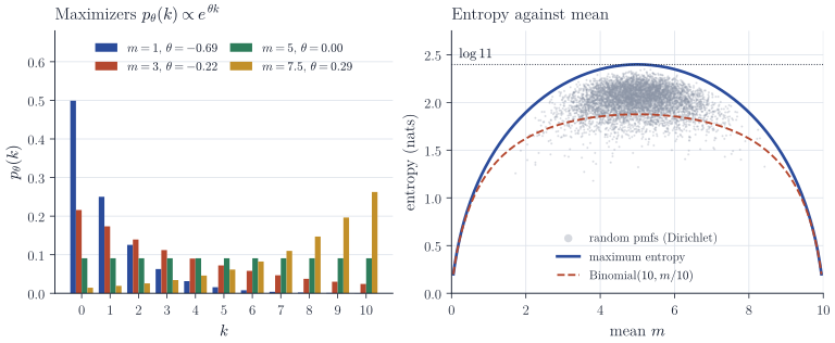
Figure 1 shows this for $\mathcal X = \{0, 1, \dots, 10\}$ with counting measure and $T(x) = x$. The maximizers are truncated geometric distributions, increasing when $m > 5$, decreasing when $m < 5$ and uniform at $m = 5$. The right panel plots entropy against the mean for random probability vectors; by Theorem 2 every one of them lies below the maximum entropy curve, and so does the binomial family.

Maximum entropy probability mass functions on zero to ten for several means, and entropy against mean for random distributions with the maximum entropy curve as upper envelope — Figure 1. Maximum entropy on $\{0,\dots,10\}$ with a mean constraint. Left: the maximizers $p_\theta(k) \propto e^{\theta k}$ for four values of the mean $m$. Right: mean and entropy of 6,000 probability vectors drawn from the uniform Dirichlet distribution (grey), the maximum entropy curve $m \mapsto A(\theta^\ast) - \theta^\ast m$ (blue), and the binomial distributions with the same mean (red, dashed).

Examples

Each of the following is an application of Theorem 2, after checking that the displayed density belongs to the family $p_\theta$ and satisfies the constraints.

Finite set, no constraint. With $T \equiv 0$ the family consists of the uniform distribution alone, so $H(p) \le \log K$ with equality only for the uniform.
Binomial distributions. On $\{0, \dots, N\}$ the binomial with mean $m$ has smaller Shannon entropy than the maximizer in Figure 1 (where $N = 10$). It is nonetheless a maximum entropy distribution, for a different reference measure: with $\mu(\{x\}) = \binom{N}{x}$ and $T(x) = x$, the density of the binomial with success probability $q$ is $p_\theta(x) = e^{\theta x}(1 + e^\theta)^{-N}$ with $\theta = \log\{q/(1-q)\}$, so it maximizes $h_\mu$ among distributions on $\{0, \dots, N\}$ with mean $Nq$.
Positive half-line, fixed mean. On $(0,\infty)$ with Lebesgue measure and $T(x) = x$, the density $m^{-1}e^{-x/m}$ has $\theta^\ast = -1/m$. The exponential distribution with mean $m$ maximizes entropy, with $h = 1 + \log m$.
Nonnegative integers, fixed mean. On $\{0, 1, 2, \dots\}$ with counting measure, the geometric distribution $p(x) = (1-q)q^x$ with $q = m/(1+m)$ has mean $m$ and $\theta^\ast = \log q$.
Real line, fixed mean and variance. With $T(x) = (x, x^2)$ and $t = (\mu, \sigma^2 + \mu^2)$, the $N(\mu, \sigma^2)$ density is of the form $p_\theta$ with $\theta^\ast = (\mu/\sigma^2, -1/(2\sigma^2))$, and $h = \tfrac12\log(2\pi e\sigma^2)$. For unit variance this is about $1.419$; the Laplace distribution with unit variance has entropy $1 + \tfrac12\log 2 \approx 1.347$ and the uniform $\tfrac12\log 12 \approx 1.242$.
Real line, fixed mean absolute value. With $T(x) = \abs{x}$ and $t = b$, the maximizer is the Laplace density $(2b)^{-1}e^{-\abs{x}/b}$.

Example 5 is the source of many extremal properties of the normal distribution. It also gives the standard bound $h(f) \le \tfrac12\log(2\pi e\,\sigma^2)$ for any density with variance $\sigma^2$, which is what makes Gaussian noise the worst case in the computation of channel capacity under a power constraint.

When the supremum is not attained

Theorem 2 says nothing when no member of the exponential family meets the constraints, and in that case the maximum may fail to exist. Here is a simple instance on $\R$ with Lebesgue measure.

Proposition 3. Let $s > 3$ and let $\mathcal G_s$ be the set of densities $f \in \mathcal F_t$ for $T(x) = (x^2, x^4)$ and $t = (1, s)$, that is, with $\int x^2 f = 1$ and $\int x^4 f = s$. Then $\sup_{f\in\mathcal G_s} h(f) = \tfrac12\log(2\pi e)$, and the supremum is not attained.

Proof. Every $f \in \mathcal G_s$ has second moment $1$, so Theorem 2 with the single statistic $x^2$ (where $\theta^\ast = -1/2$ and the maximizer is the $N(0,1)$ density) gives $h(f) \le \tfrac12\log(2\pi e)$, with equality only for $N(0,1)$. The standard normal has fourth moment $3 \ne s$, so the bound is not attained on $\mathcal G_s$.

To show that the bound is approached, let $\phi_v$ be the $N(0, v)$ density and consider mixtures $f = (1-\varepsilon)\phi_{\sigma^2} + \varepsilon\phi_{\tau^2}$. The constraints read $(1-\varepsilon)\sigma^2 + \varepsilon\tau^2 = 1$ and $3(1-\varepsilon)\sigma^4 + 3\varepsilon\tau^4 = s$. Fix $\tau^2 > 1$ large, write $u = \varepsilon\tau^2$, and eliminate $\sigma^2 = (1-u)/(1-\varepsilon)$; the second constraint becomes

\[G(u) := \frac{(1-u)^2}{1 - u/\tau^2} + u\,\tau^2 = \frac{s}{3} .\]

$G$ is continuous on $[0, 1)$, $G(0) = 1 < s/3$, and $G(u) > s/3$ at $u = s/(3\tau^2)$, which lies in $(0,1)$ once $\tau^2 > s/3$. So a solution $u_\tau \in (0, s/(3\tau^2))$ exists, and with $\varepsilon_\tau = u_\tau/\tau^2 \le s/(3\tau^4)$ we get $\sigma_\tau^2 = (1 - u_\tau)/(1 - \varepsilon_\tau) \to 1$ as $\tau \to \infty$.

Entropy is concave: the function $y \mapsto -y\log y$ is concave on $[0,\infty)$, so pointwise $-f\log f \ge -(1-\varepsilon)\phi_{\sigma^2}\log\phi_{\sigma^2} - \varepsilon\,\phi_{\tau^2}\log\phi_{\tau^2}$, and integrating (all terms are integrable for Gaussian mixtures),

\[h(f) \ge (1-\varepsilon_\tau)\,\tfrac12\log(2\pi e\,\sigma_\tau^2) + \varepsilon_\tau\,\tfrac12\log(2\pi e\,\tau^2) .\]

As $\tau \to \infty$ the first term tends to $\tfrac12\log(2\pi e)$, and the second is at most $\tfrac{s}{6\tau^4}\log(2\pi e\tau^2) \to 0$ in absolute value.

The maximizing sequence keeps the bulk of its mass close to $N(0,1)$ and places a vanishing fraction $\varepsilon_\tau$ of it far out, where it supplies the excess fourth moment at negligible cost in entropy. The proposition also shows indirectly that no density of the form $\exp(\theta_1 x^2 + \theta_2 x^4 - A(\theta))$ has second moment 1 and fourth moment $s > 3$: if one did, Theorem 2 would make it a maximizer.

Remarks

Theorem 2 is the special case of a more general fact about minimizing $\KL(f\,\Vert\,g)$ over a convex set of densities $f$ (the maximum entropy problem takes $g$ to be the uniform density when $\mu$ is finite). This is the theory of I-projections developed by I. Csiszár, “I-divergence geometry of probability distributions and minimization problems” (Annals of Probability, 1975). The Lagrangian heuristic above also has a rigorous counterpart: the dual of the maximum entropy problem is maximum likelihood in the exponential family $p_\theta$, a relation that is the subject of a companion note.

Jaynes’s argument for the principle appears in “Information theory and statistical mechanics” (Physical Review, 1957), and T. M. Cover and J. A. Thomas, Elements of Information Theory, has a chapter on maximum entropy with many further examples.