Natural gradient descent: steepest descent measured by the Fisher information
“The gradient points in the direction of steepest ascent” is true only after a choice of how to measure the length of a step. The usual choice, Euclidean length in the coordinates at hand, is harmless when the coordinates are arbitrary labels of points in space. When the coordinates parametrize probability distributions, it is an artefact: a change of \(0.1\) in a location parameter is a large change in the distribution if the scale is \(0.01\) and a negligible one if the scale is \(100\). Natural gradient methods measure step lengths by how much the distribution changes, and the resulting update is the same whichever parametrization of the model is used.
Steepest descent depends on the metric
Let \(L : \Theta \to \R\) be differentiable on an open set \(\Theta \subseteq \R^d\), with gradient \(g = \nabla L(\theta)\) at the current point. If step lengths are measured by \(\lVert\delta\rVert_M = (\delta^\top M\delta)^{1/2}\) for a positive definite matrix \(M\), the best first-order decrease within a step of length \(\varepsilon\) is obtained by minimizing \(g^\top\delta\) subject to \(\delta^\top M \delta \le \varepsilon^2\). By the Cauchy–Schwarz inequality,
\[g^\top \delta = (M^{-1/2}g)^\top (M^{1/2}\delta) \ge -\lVert M^{-1/2}g\rVert\, \lVert M^{1/2}\delta\rVert \ge -\varepsilon\,(g^\top M^{-1} g)^{1/2},\]with equality exactly when \(M^{1/2}\delta\) is a nonpositive multiple of \(M^{-1/2}g\) of norm \(\varepsilon\). The minimizer is
\[\delta^\star = -\varepsilon\, \frac{M^{-1}g}{(g^\top M^{-1}g)^{1/2}} .\]So the steepest descent direction is \(-M^{-1}g\), not \(-g\); the vector \(M^{-1}g\) is the gradient of \(L\) with respect to the inner product \(\langle u, v\rangle_M = u^\top Mv\). Ordinary gradient descent is the case \(M = I\), and Newton’s method can be read as the case \(M = \nabla^2 L(\theta)\) when the Hessian is positive definite. The question is which \(M\) is natural when \(\theta\) indexes a family of distributions.
The Fisher information as a local metric
Let \(\{p_\theta : \theta \in \Theta\}\) be densities with respect to a common measure \(\nu\), and assume:
- \(\theta \mapsto \log p_\theta(x)\) is twice continuously differentiable for every \(x\);
- differentiation under the integral sign is permitted twice in \(\int p_\theta\, \dd\nu = 1\) and in \(\theta' \mapsto \int p_\theta \log p_{\theta'}\, \dd\nu\) near \(\theta' = \theta\) (for instance, the derivatives are dominated by \(\nu\)-integrable functions locally uniformly), and the resulting second derivative is continuous in \(\theta'\);
- the Fisher information \(F(\theta) = \E_\theta\bigl[\nabla\log p_\theta(X)\, \nabla\log p_\theta(X)^\top\bigr]\) is finite and positive definite.
Lemma 1. Under these assumptions, as \(\delta \to 0\),
\[\KL(p_\theta \,\Vert\, p_{\theta+\delta}) = \tfrac12\, \delta^\top F(\theta)\, \delta + o(\lVert\delta\rVert^2).\]Proof. Let \(K(\theta') = \KL(p_\theta \Vert p_{\theta'}) = \E_\theta \log p_\theta(X) - \E_\theta \log p_{\theta'}(X)\). Then \(K(\theta) = 0\). Differentiating under the integral sign, \(\nabla K(\theta) = -\E_\theta \nabla\log p_\theta(X) = -\int \nabla p_\theta\, \dd\nu = -\nabla \int p_\theta\, \dd\nu = 0\), and \(\nabla^2 K(\theta) = -\E_\theta \nabla^2 \log p_\theta(X)\). Differentiating the identity \(\int (\nabla \log p_\theta)\, p_\theta\, \dd\nu = 0\) once more gives \(\E_\theta\nabla^2\log p_\theta + \E_\theta[\nabla\log p_\theta\nabla\log p_\theta^\top] = 0\), so \(\nabla^2 K(\theta) = F(\theta)\). Taylor’s theorem with the continuity of \(\nabla^2 K\) at \(\theta\) gives the expansion.
Under the analogous conditions with the roles of the two arguments exchanged, the same expansion holds for \(\KL(p_{\theta+\delta}\Vert p_\theta)\), so to second order the asymmetry of the divergence disappears. The Fisher information is the metric that the family of distributions induces on its parameter space, the Fisher–Rao metric. Replacing the Euclidean constraint by \(\KL(p_\theta \Vert p_{\theta+\delta}) \le \varepsilon^2/2\) and using Lemma 1, the constraint becomes \(\delta^\top F(\theta)\delta \le \varepsilon^2(1 + o(1))\), and the steepest descent direction, to leading order as \(\varepsilon \to 0\), is \(-F(\theta)^{-1}\nabla L(\theta)\).
Definition 2. The natural gradient of \(L\) at \(\theta\) is \(\tilde\nabla L(\theta) = F(\theta)^{-1}\nabla L(\theta)\), and natural gradient descent is the iteration \(\theta_{k+1} = \theta_k - \eta_k\, F(\theta_k)^{-1}\nabla L(\theta_k)\).
The idea is due to Amari (“Natural gradient works efficiently in learning”, Neural Computation, 1998). For the normal family \(N(\mu, \sigma^2)\) with \(\theta = (\mu, \sigma)\), the score is \(\bigl((x-\mu)/\sigma^2,\, -1/\sigma + (x-\mu)^2/\sigma^3\bigr)\), and using \(\E(X-\mu)^2 = \sigma^2\), \(\E(X - \mu)^3 = 0\) and \(\E(X-\mu)^4 = 3\sigma^4\),
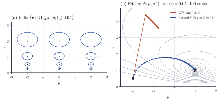
\[F(\mu, \sigma) = \begin{pmatrix} 1/\sigma^2 & 0 \\ 0 & 2/\sigma^2 \end{pmatrix}.\]The metric \((\dd\mu^2 + 2\,\dd\sigma^2)/\sigma^2\) becomes \(2(\dd u^2 + \dd\sigma^2)/\sigma^2\) in the coordinate \(u = \mu/\sqrt2\), a constant multiple of the metric of the hyperbolic upper half-plane. Panel (a) of Figure 1 shows what this means: sets of distributions within a fixed Kullback–Leibler divergence of a centre are small near \(\sigma = 0\) and large for large \(\sigma\), so a fixed Euclidean step is enormous in the first case and negligible in the second.
Invariance under reparametrization
Let \(\theta = \varphi(\xi)\) with \(\varphi\) a diffeomorphism between open sets, \(J(\xi) = D\varphi(\xi)\) its Jacobian, and \(\tilde L = L \circ \varphi\). The model in the new coordinates has densities \(p_{\varphi(\xi)}\).
Proposition 3. The Fisher information in \(\xi\) is \(\tilde F(\xi) = J^\top F(\varphi(\xi))\, J\), and the natural gradients satisfy
\[J(\xi)\, \tilde F(\xi)^{-1}\nabla_\xi \tilde L(\xi) = F(\theta)^{-1}\nabla_\theta L(\theta), \qquad \theta = \varphi(\xi).\]Consequently, if \(\xi(t)\) solves \(\dot\xi = -\tilde F(\xi)^{-1}\nabla_\xi\tilde L(\xi)\), then \(\theta(t) = \varphi(\xi(t))\) solves \(\dot\theta = -F(\theta)^{-1}\nabla_\theta L(\theta)\).
Proof. By the chain rule, \(\nabla_\xi \log p_{\varphi(\xi)} = J^\top \nabla_\theta\log p_\theta\) and \(\nabla_\xi\tilde L = J^\top\nabla_\theta L\). Taking the expected outer product of the first identity gives \(\tilde F = J^\top F J\). Since \(J\) is invertible, \(\tilde F^{-1}\nabla_\xi\tilde L = J^{-1}F^{-1}J^{-\top}J^\top\nabla_\theta L = J^{-1}F^{-1}\nabla_\theta L\). For the flows, \(\dot\theta = J\dot\xi = -F^{-1}\nabla_\theta L\).
The natural gradient therefore transforms like a velocity vector, and the continuous-time natural gradient flow traces the same curve of distributions in every parametrization. Ordinary gradient flow does not: in \(\xi\) coordinates it produces \(\dot\theta = -JJ^\top\nabla_\theta L\), which depends on \(\varphi\) unless \(J\) is orthogonal. For discrete steps the invariance holds only to first order in the step size, since \(\varphi(\xi - \eta d)\) and \(\varphi(\xi) - \eta J d\) differ at order \(\eta^2\).
Maximum likelihood for the normal family
Let \(L(\mu, \sigma)\) be the average negative log-likelihood of observations with sample mean \(\bar x\) and mean squared deviation \(s^2\):
\[L(\mu, \sigma) = \log\sigma + \frac{s^2 + (\bar x - \mu)^2}{2\sigma^2} + \text{const}, \qquad \nabla L = \begin{pmatrix} -(\bar x - \mu)/\sigma^2 \\ 1/\sigma - (s^2 + (\bar x - \mu)^2)/\sigma^3 \end{pmatrix}.\]Gradient descent moves \(\mu\) by \(\eta(\bar x - \mu)/\sigma^2\), which explodes as \(\sigma \to 0\), and moves \(\sigma\) by an amount of order \(\sigma^{-3}\) when \(\sigma\) is small. The natural gradient step is
\[\mu \leftarrow \mu + \eta(\bar x - \mu), \qquad \sigma \leftarrow \sigma + \frac{\eta\,\sigma}{2}\Bigl(\frac{s^2 + (\bar x-\mu)^2}{\sigma^2} - 1\Bigr),\]in which \(\mu\) moves a fixed fraction of the way to \(\bar x\) whatever the scale, and \(\sigma\) changes by a relative amount. Panel (b) of Figure 1 runs both from \((\mu, \sigma) = (-2, 0.5)\) with the same step size. The first gradient step is dominated by the \(\sigma\)-component and throws the iterate to \(\sigma \approx 4.4\), where all gradients are small and progress is slow; the natural gradient iterates move steadily to the maximum likelihood estimate.
Exponential families: natural gradients are mean-parameter gradients
Let \(p_\theta(x) = h(x)\exp\bigl(\theta^\top T(x) - A(\theta)\bigr)\) be a minimal exponential family with natural parameter \(\theta\) in an open set, so that \(A\) is smooth and \(\nabla^2 A(\theta) = \Cov_\theta T(X)\) is positive definite. The mean parameter is \(m(\theta) = \nabla A(\theta) = \E_\theta T(X)\), and \(F(\theta) = \nabla^2 A(\theta)\). For data with average sufficient statistic \(\bar T\), the average negative log-likelihood is \(L(\theta) = A(\theta) - \theta^\top \bar T\) up to a constant, so
\[\nabla L(\theta) = m(\theta) - \bar T, \qquad \nabla^2 L(\theta) = F(\theta), \qquad \tilde\nabla L(\theta) = F(\theta)^{-1}\bigl(m(\theta) - \bar T\bigr).\]Three readings of the last expression follow.
- Newton’s method. Because the Hessian of \(L\) equals the Fisher information, natural gradient descent with \(\eta = 1\) is Newton’s method, and in generalized linear models with canonical link it is Fisher scoring, that is, iteratively reweighted least squares. More generally, Fisher scoring \(\theta \leftarrow \theta + F(\theta)^{-1}\nabla \ell_n(\theta)/n\) for any regular model is natural gradient ascent on the average log-likelihood \(\ell_n/n\) with unit step.
- Gradient in mean coordinates. The map \(\theta \mapsto m(\theta)\) is a diffeomorphism onto its image with Jacobian \(F(\theta)\). By the chain rule, the gradient of \(L\) with respect to \(m\) is \(F(\theta)^{-1}\nabla_\theta L = \tilde\nabla L(\theta)\): the natural gradient in natural coordinates is the ordinary gradient in mean coordinates.
- Straight lines in the mean. Along the natural gradient flow \(\dot\theta = -F^{-1}(m - \bar T)\), the mean parameter satisfies \(\dot m = F\dot\theta = -(m - \bar T)\), so \(m(t) = \bar T + e^{-t}(m(0) - \bar T)\): the flow moves the mean parameter along a straight line towards the data, at an exponential rate that does not depend on the curvature of \(A\). (The solution requires the segment to stay among the attainable means. When \(\theta\) ranges over the whole natural parameter space and that space is open, the attainable means form the interior of the convex hull of the support of \(T(X)\), a convex set, so it suffices that \(\bar T\) lies in that interior.)
The second fact is behind the simple form of natural-gradient updates in stochastic variational inference for conditionally conjugate models (Hoffman, Blei, Wang and Paisley, Journal of Machine Learning Research, 2013), where the natural gradient of the evidence lower bound with respect to the natural parameters of an exponential-family factor is the difference between a target natural parameter and the current one.
Remarks
In models where \(F(\theta)\) is not available in closed form, it must be estimated or approximated, and the choice matters. The Fisher information is an expectation under the model; replacing it by the average of outer products of per-observation gradients at the observed data, the so-called empirical Fisher, gives a different matrix that agrees with \(F\) only under correct specification and near the optimum, and it can produce poor directions elsewhere. For neural networks, Kronecker-factored approximations of the Fisher information (Martens and Grosse, 2015) make natural gradient steps affordable. In the other direction, the Fisher–Rao metric is the starting point of information geometry, in which exponential families are dually flat, with the natural and the mean parameters as the two affine coordinate systems; Amari, Information Geometry and Its Applications, develops that theory.