Gaussians with a random variance: the Laplace and Student-t distributions as normal scale mixtures
A normal observation whose variance is itself random is no longer normal. Mixing over the variance thickens the tails while keeping the distribution symmetric and unimodal, and two of the most common heavy-tailed laws in statistics arise exactly this way: the Laplace distribution, behind the lasso and least absolute deviations, and the Student-t, behind robust regression. The representation is useful in two directions. It explains where the tails come from, and conditionally on the variance everything is Gaussian again, which is what makes EM algorithms and Gibbs samplers for these models simple.
Normal scale mixtures
Let \(Z \sim N(0,1)\) and let \(V\) be a random variable with \(\P(V > 0) = 1\), independent of \(Z\). The law of
\[X = \sqrt V\,Z\]is called a normal scale mixture with mixing distribution the law of \(V\). Conditionally on \(V = v\), \(X \sim N(0, v)\). Write \(\phi_v(x) = (2\pi v)^{-1/2}e^{-x^2/(2v)}\).
Proposition 1. Let \(X = \sqrt V Z\) be a normal scale mixture.
- \(X\) has the density \(f(x) = \E\,\phi_V(x)\), which is symmetric and nonincreasing in \(\abs{x}\).
- The characteristic function of \(X\) is \(\E e^{\mathrm{i}tX} = \E e^{-t^2V/2}\), the Laplace transform of \(V\) evaluated at \(t^2/2\).
- \(\E X^2 = \E V\). If \(\E V^2 < \infty\), the kurtosis \(\E X^4/(\E X^2)^2\) equals \(3\,\E V^2/(\E V)^2 \ge 3\), with equality if and only if \(V\) is almost surely constant.
Proof. For a Borel set \(A\), conditioning on \(V\) and Tonelli’s theorem (the integrand is nonnegative) give \(\P(X \in A) = \E\int_A\phi_V(x)\,\dd x = \int_A\E\,\phi_V(x)\,\dd x\). Each \(\phi_v\) is symmetric and nonincreasing in \(\abs{x}\), and both properties survive averaging over \(v\). Part 2 follows from \(\E[e^{\mathrm{i}tX} \mid V] = e^{-t^2V/2}\). For part 3, independence gives \(\E X^2 = \E V\,\E Z^2\) and \(\E X^4 = \E V^2\,\E Z^4 = 3\E V^2\), and \((\E V)^2 \le \E V^2\) with equality exactly when \(\Var V = 0\).
Part 3 already rules out many symmetric laws. The uniform distribution on \((-1,1)\) has kurtosis \(9/5 < 3\), so it is not a normal scale mixture, whatever the mixing distribution. Scale mixing can only add kurtosis.
The tails of \(X\) are governed by the right tail of \(V\). For \(x > 0\), on the event \(\{V > x^2\} \cap \{\abs{Z} > 1\}\) we have \(\abs{X} > x\), so by independence
\[\P(\abs{X} > x) \ge \P(\abs{Z} > 1)\,\P(V > x^2) \approx 0.317\,\P(V > x^2).\]A mixing distribution with polynomial tail \(\P(V > v) \approx c\,v^{-\alpha}\) therefore forces a polynomial tail of order at least \(x^{-2\alpha}\) in \(X\). In the other direction, \(\abs{X} > x\) implies \(V > x\) or \(\abs{Z} > \sqrt x\) (otherwise \(\abs{X} \le \sqrt x\cdot\sqrt x\)), so
\[\P(\abs{X} > x) \le \P(V > x) + \P(\abs{Z} > \sqrt x),\]and a mixing distribution with an exponential tail \(\P(V > v) \le Ce^{-cv}\) produces at most exponential tails in \(X\).
The Laplace distribution
The Laplace distribution with scale \(b > 0\) has density \((2b)^{-1}e^{-\abs{x}/b}\) and characteristic function
\[\int_{-\infty}^\infty e^{\mathrm{i}tx}\,\frac{e^{-\abs{x}/b}}{2b}\,\dd x = \frac1{2b}\Bigl(\frac{1}{1/b - \mathrm{i}t} + \frac{1}{1/b + \mathrm{i}t}\Bigr) = \frac{1}{1 + b^2t^2} .\]Proposition 2. If \(V\) is exponential with mean \(2b^2\), then \(\sqrt V Z\) has the Laplace distribution with scale \(b\).
Proof. The Laplace transform of an exponential variable with rate \(\lambda\) is \(\E e^{-sV} = \lambda/(\lambda + s)\) for \(s \ge 0\). With \(\lambda = 1/(2b^2)\) and \(s = t^2/2\), part 2 of Proposition 1 gives
\[\E e^{\mathrm{i}t\sqrt V Z} = \frac{1/(2b^2)}{1/(2b^2) + t^2/2} = \frac{1}{1 + b^2t^2},\]which is the Laplace characteristic function. Characteristic functions determine distributions.
Since \(\E V = 2b^2\) and \(\E V^2 = 8b^4\), Proposition 1 gives variance \(2b^2\) and kurtosis \(3 \cdot 8b^4/(4b^4) = 6\), the known values for the Laplace law.
The Student-t distribution
Recall that \(t_\nu\), the Student-t distribution with \(\nu > 0\) degrees of freedom, has density
\[f_\nu(x) = \frac{\Gamma\bigl(\frac{\nu+1}{2}\bigr)}{\sqrt{\nu\pi}\,\Gamma\bigl(\frac\nu2\bigr)}\Bigl(1 + \frac{x^2}{\nu}\Bigr)^{-(\nu+1)/2} .\]Proposition 3. Let \(G\) have the \(\chi^2_\nu\) distribution, that is, the gamma distribution with shape \(\nu/2\) and rate \(1/2\), independent of \(Z\). Then \(X = \sqrt{\nu/G}\,Z\) has the \(t_\nu\) distribution. Equivalently, \(t_\nu\) is the normal scale mixture whose precision \(1/V\) is gamma with shape \(\nu/2\) and rate \(\nu/2\).
Proof. By part 1 of Proposition 1 with \(V = \nu/G\), the density of \(X\) is
\[\begin{aligned} f(x) &= \int_0^\infty \sqrt{\frac{g}{2\pi\nu}}\,e^{-x^2g/(2\nu)}\,\frac{g^{\nu/2 - 1}e^{-g/2}}{2^{\nu/2}\Gamma(\nu/2)}\,\dd g \\ &= \frac{(2\pi\nu)^{-1/2}}{2^{\nu/2}\Gamma(\nu/2)}\int_0^\infty g^{\frac{\nu+1}{2} - 1}\exp\Bigl\{-\frac g2\Bigl(1 + \frac{x^2}{\nu}\Bigr)\Bigr\}\,\dd g . \end{aligned}\]The last integral is a gamma integral, equal to \(\Gamma\bigl(\frac{\nu+1}2\bigr)\bigl(2/(1 + x^2/\nu)\bigr)^{(\nu+1)/2}\). Collecting the powers of two, \((2\pi\nu)^{-1/2}\,2^{(\nu+1)/2}/2^{\nu/2} = (\pi\nu)^{-1/2}\), which gives \(f = f_\nu\). The second statement is the observation that \(G/\nu\) has shape \(\nu/2\) and rate \(\nu/2\).
The mixing variable \(V = \nu/G\) is inverse-gamma, with \(\P(V > v) = \P(G < \nu/v) \sim c\,v^{-\nu/2}\) as \(v \to \infty\), because the \(\chi^2_\nu\) density behaves like a multiple of \(g^{\nu/2-1}\) near zero. The lower bound above then gives a tail of order \(x^{-\nu}\) for \(X\), which matches the exact behaviour of \(t_\nu\): integrating \(f_\nu\) gives \(\P(\abs{X} > x) \sim c'\,x^{-\nu}\). For \(\nu = 1\) this is the Cauchy distribution. Moments of \(X\) of order \(k\) exist exactly when \(k < \nu\), which by independence is the condition \(\E V^{k/2} < \infty\).
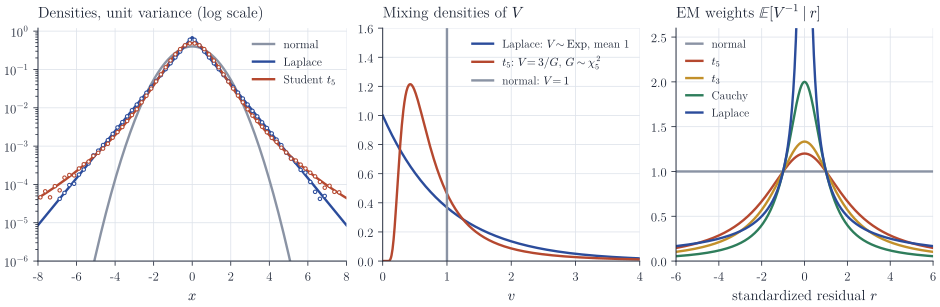
Figure 1 compares the three laws standardized to unit variance: the Laplace distribution with \(b = 1/\sqrt2\), and \(t_5\) rescaled by \(\sqrt{3/5}\), whose mixing variable is \(V = 3/G\) with \(G \sim \chi^2_5\). All three mixing distributions have mean one; they differ in how much mass they put on large variances.
Conditional conjugacy and reweighting
Given \(V\), an observation is Gaussian, and given an observation, the mixing variable often has a tractable posterior. For the \(t\) distribution, write \(\lambda = 1/V\) for the precision.
Proposition 4. If \(\lambda\) is gamma with shape \(\nu/2\) and rate \(\nu/2\) and, given \(\lambda\), \(X \sim N(0, 1/\lambda)\), then given \(X = x\) the precision is gamma with shape \((\nu+1)/2\) and rate \((\nu + x^2)/2\). In particular \(\E[\lambda \mid X = x] = (\nu+1)/(\nu + x^2)\).
Proof. The joint density of \((\lambda, X)\) is proportional to \(\lambda^{1/2}e^{-\lambda x^2/2}\cdot\lambda^{\nu/2 - 1}e^{-\nu\lambda/2} = \lambda^{(\nu+1)/2 - 1}e^{-\lambda(\nu + x^2)/2}\), which as a function of \(\lambda\) is the stated gamma kernel. The mean of a gamma variable is shape divided by rate.
For the Laplace distribution the posterior of \(V\) given \(X = x \ne 0\) is proportional to \(v^{-1/2}\exp\{-x^2/(2v) - v/(2b^2)\}\), a generalized inverse Gaussian law. Its inverse moment follows from two integrals, valid for \(a, c > 0\):
\[\int_0^\infty v^{-1/2}e^{-a/v - cv}\,\dd v = \sqrt{\frac\pi c}\,e^{-2\sqrt{ac}}, \qquad \int_0^\infty v^{-3/2}e^{-a/v - cv}\,\dd v = \sqrt{\frac\pi a}\,e^{-2\sqrt{ac}} .\]The first is standard (it is the normalizing constant of the inverse Gaussian distribution), and the substitution \(v = a/(cu)\) turns the second into \(\sqrt{c/a}\) times the first. With \(a = x^2/2\) and \(c = 1/(2b^2)\) the ratio gives \(\E[V^{-1} \mid X = x] = \sqrt{c/a} = 1/(b\abs{x})\).
These conditional expectations are the weights of an EM algorithm. Consider a location-scale model \(x_i = \mu + \sigma\sqrt{V_i}\,Z_i\), \(i = 1, \dots, n\), with independent mixing variables. Treating the \(V_i\) as missing data, the complete-data log-likelihood is, up to terms not involving \((\mu, \sigma)\),
\[-n\log\sigma - \frac{1}{2\sigma^2}\sum_{i=1}^n V_i^{-1}(x_i - \mu)^2 ,\]which is linear in the \(V_i^{-1}\). The E-step replaces \(V_i^{-1}\) by \(w_i = \E[V_i^{-1} \mid x_i]\) evaluated at the standardized residual \(r_i = (x_i - \mu)/\sigma\), and the M-step is weighted least squares:
\[\mu \leftarrow \frac{\sum_i w_i x_i}{\sum_i w_i}, \qquad \sigma^2 \leftarrow \frac1n\sum_i w_i(x_i - \mu)^2 .\]The general theory of EM guarantees that the observed-data likelihood does not decrease along the iterations. For the \(t_\nu\) model with known \(\nu\), \(w_i = (\nu+1)/(\nu + r_i^2)\) is bounded and decreases like \(r_i^{-2}\), so outlying observations are smoothly downweighted; as \(\nu \to \infty\) the weights tend to one and the algorithm returns the sample mean and variance. For the Laplace model with \(b = 1\), \(w_i = 1/\abs{r_i}\) and the iteration is the classical reweighting scheme for least absolute deviations; the weight is undefined when a residual is exactly zero, and implementations replace \(\abs{r_i}\) by \(\max(\abs{r_i}, \epsilon)\) for a small \(\epsilon > 0\). The right panel of Figure 1 compares the weight functions. Replacing the location \(\mu\) by a regression function \(x_i^\top\beta\) changes only the M-step, which becomes a weighted least squares regression.
In Bayesian computation the same structure gives Gibbs samplers in which every full conditional is standard: given the \(V_i\) the model is Gaussian, and given the data and parameters the \(V_i\) are conditionally independent with gamma (for \(t\)) or generalized inverse Gaussian (for Laplace) laws. The Bayesian lasso of T. Park and G. Casella (Journal of the American Statistical Association, 2008) uses the Laplace mixture in this way for the regression coefficients rather than for the errors.
Remarks
Which symmetric distributions are normal scale mixtures? Writing the mixture density as \(f(\sqrt y) = \E\bigl[(2\pi V)^{-1/2}e^{-y/(2V)}\bigr]\) shows that \(y \mapsto f(\sqrt y)\) is a Laplace transform, hence completely monotone on \((0, \infty)\); by Bernstein’s theorem the converse holds as well. This characterization is due to D. F. Andrews and C. L. Mallows, “Scale mixtures of normal distributions” (Journal of the Royal Statistical Society, Series B, 1974). The EM algorithm for the \(t\) model is developed in K. L. Lange, R. J. A. Little and J. M. G. Taylor, “Robust statistical modeling using the t distribution” (Journal of the American Statistical Association, 1989).
The idea extends in several directions: letting the mean also depend on \(V\) gives normal variance-mean mixtures, including the generalized hyperbolic family; and putting a heavy-tailed mixing distribution on the scale of a regression coefficient gives shrinkage priors such as the horseshoe.