Normalizing flows: exact densities through invertible maps

Most flexible density models give up something: mixtures and latent-variable models have intractable marginal likelihoods, and energy-based models have intractable normalizing constants. A normalizing flow keeps the likelihood exact by construction. One fixes a simple base density $p_U$ on $\R^d$, usually $\mathcal N(0, I_d)$, and models data as $X = T(U)$ for an invertible map $T$. Sampling is then a forward pass through $T$, and the density of $X$ follows from the change-of-variables formula, provided the Jacobian determinant of $T$ can be computed. The design problem is to make $T$ flexible while keeping both its inverse and its Jacobian determinant cheap. Triangular maps solve it, and maximum likelihood fitting of the resulting models is a Kullback–Leibler projection that can be read either in the data space or in the base space.

Change of variables

Theorem 1. Let $\mathcal U, \mathcal X \subseteq \R^d$ be open and let $T : \mathcal U \to \mathcal X$ be a continuously differentiable bijection whose Jacobian matrix $J_T(u)$ is nonsingular for every $u \in \mathcal U$. If $U$ has density $p_U$ on $\mathcal U$, then $X = T(U)$ has density

\[p_X(x) = p_U\bigl(T^{-1}(x)\bigr)\,\bigl\lvert \det J_{T^{-1}}(x) \bigr\rvert = \frac{p_U(u)}{\lvert \det J_T(u) \rvert}, \qquad u = T^{-1}(x),\ x \in \mathcal X,\]

and $p_X = 0$ outside $\mathcal X$.

Proof. By the inverse function theorem, $T^{-1}$ is continuously differentiable, so $T$ is a $C^1$ diffeomorphism, and differentiating $T(T^{-1}(x)) = x$ gives $J_{T^{-1}}(x) = J_T(u)^{-1}$. For a Borel set $A \subseteq \mathcal X$, $\P(X \in A) = \int_{T^{-1}(A)} p_U(u)\,\dd u$. The change-of-variables theorem for Lebesgue integrals, applied to the diffeomorphism $T^{-1} : \mathcal X \to \mathcal U$ and the nonnegative function $p_U \mathbf 1_{T^{-1}(A)}$, gives

\[\int_{T^{-1}(A)} p_U(u)\,\dd u = \int_{\mathcal X} p_U\bigl(T^{-1}(x)\bigr)\, \mathbf 1_A(x)\, \bigl\lvert \det J_{T^{-1}}(x)\bigr\rvert\, \dd x ,\]

which identifies the density.

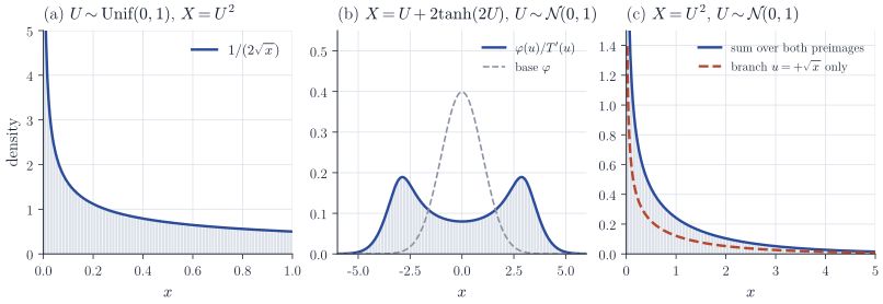
The factor $\lvert \det J_T(u) \rvert$ is the local volume expansion of $T$ at $u$: where the map stretches space, probability is spread thinner. Figure 1 shows three one-dimensional cases. In panel (a), $T(u) = u^2$ is a diffeomorphism of $(0,1)$ onto itself and the uniform base becomes the density $1/(2\sqrt x)$. In panel (b), $T(u) = u + 2\tanh(2u)$ has $T'(u) = 1 + 4\operatorname{sech}^2(2u) \in [1, 5]$ and is a diffeomorphism of $\R$; it stretches a neighbourhood of the origin by a factor close to $5$, so the unimodal Gaussian becomes bimodal, with $p_X(0) = \varphi(0)/5 \approx 0.08$. Panel (c) shows what the hypotheses exclude. The map $u \mapsto u^2$ on $\R$ is two-to-one; applying the theorem separately on $(-\infty, 0)$ and $(0, \infty)$ and adding the two contributions gives the $\chi^2_1$ density $\varphi(\sqrt x)/\sqrt x$, and using a single branch loses half of the mass.

Three panels comparing histograms of transformed samples with the densities given by the change-of-variables formula — Figure 1. Histograms of $10^5$ draws of $X = T(U)$ and the densities from Theorem 1. (a) $U$ uniform on $(0,1)$, $T(u) = u^2$. (b) $U \sim \mathcal N(0,1)$, $T(u) = u + 2\tanh(2u)$; the curve is drawn parametrically as $u \mapsto (T(u), \varphi(u)/T'(u))$, which avoids inverting $T$, and the dashed curve is the base density $\varphi$. (c) $U \sim \mathcal N(0,1)$ and the non-injective map $u \mapsto u^2$: the correct density sums over both preimages.

Flows are built by composition. If $T = T_K \circ \cdots \circ T_1$ with each $T_k$ as in Theorem 1, and $z_0 = u$, $z_k = T_k(z_{k-1})$, then the chain rule and multiplicativity of the determinant give

\[\begin{equation} \log p_X(x) = \log p_U(u) - \sum_{k=1}^K \log\bigl\lvert \det J_{T_k}(z_{k-1})\bigr\rvert, \qquad u = T^{-1}(x). \label{eq:composition} \end{equation}\]

A general $d \times d$ determinant costs $O(d^3)$ operations, and a general nonlinear map has no closed-form inverse. Both problems disappear for triangular maps.

Triangular maps

Call $T$ lower triangular if its $i$th coordinate depends only on the first $i$ inputs, $x_i = T_i(u_1, \dots, u_i)$. Then $J_T$ is lower triangular and

\[\det J_T(u) = \prod_{i=1}^d \frac{\partial T_i}{\partial u_i}(u_1, \dots, u_i).\]

If, in addition, each $u_i \mapsto T_i(u_1, \dots, u_{i-1}, u_i)$ is a strictly increasing bijection of $\R$, then $T$ is a bijection, inverted one coordinate at a time: $u_1$ is recovered from $x_1$, then $u_2$ from $(u_1, x_2)$, and so on. Restricting to such maps loses nothing in principle.

Proposition 2 (Knothe–Rosenblatt map). Let $p$ be a probability density on $\R^d$ with $p(x) > 0$ for all $x$. There is a lower triangular Borel map $T : \R^d \to \R^d$, with each $T_i$ strictly increasing in $u_i$, such that $T(U)$ has density $p$ when $U \sim \mathcal N(0, I_d)$.

Proof. Let $p_{1:i}(x_{1:i}) = \int p(x_{1:i}, y)\,\dd y$ (integral over $\R^{d-i}$) be the marginal density of the first $i$ coordinates. By Tonelli’s theorem it is Borel, takes values in $(0, \infty]$ because $p > 0$, is finite outside a Lebesgue-null set $N_i$, and satisfies $\int p_{1:i}(x_{1:i-1}, s)\,\dd s = p_{1:i-1}(x_{1:i-1})$ for every $x_{1:i-1}$. For $x_{1:i-1} \notin N_{i-1}$ let

\[F_i(t \mid x_{1:i-1}) = \frac{1}{p_{1:i-1}(x_{1:i-1})} \int_{-\infty}^t p_{1:i}(x_{1:i-1}, s)\,\dd s\]

be the conditional distribution function of the $i$th coordinate (with $F_1$ the marginal distribution function of the first), and on $N_{i-1}$ set $F_i(t \mid x_{1:i-1}) = \Phi(t)$, where $\Phi$ is the standard normal distribution function. It is Borel in $x_{1:i-1}$ for each $t$ by Tonelli’s theorem and continuous in $t$, hence jointly Borel, and it is strictly increasing in $t$ with limits $0$ and $1$, so its inverse in $t$ exists; the inverse is jointly Borel because $\{F_i^{-1}(v \mid x_{1:i-1}) \le t\} = \{v \le F_i(t \mid x_{1:i-1})\}$. Define recursively $x_i = F_i^{-1}(\Phi(u_i) \mid x_{1:i-1})$. Since $\Phi(U_i)$ is uniform on $(0,1)$ and independent of $(U_1, \dots, U_{i-1})$, which determine $x_{1:i-1}$, the inverse-transform method shows that the conditional law of $X_i$ given $X_{1:i-1}$ has distribution function $F_i(\cdot \mid X_{1:i-1})$. If $X_{1:i-1}$ has density $p_{1:i-1}$, it avoids the null set $N_{i-1}$ almost surely, and this conditional distribution function has density $p_{1:i}(X_{1:i-1}, \cdot)/p_{1:i-1}(X_{1:i-1})$, so $X_{1:i}$ has density $p_{1:i}$. By induction on $i$ this holds for $i = d$, which is the claim.

The construction is explicit, but it uses conditional distribution functions that are unavailable in practice. Flows parametrize triangular maps directly instead, in two main ways.

Coupling layers

Split the coordinates into a block $A$ of size $k$ and its complement $B$. An affine coupling layer leaves $u_A$ unchanged and transforms $u_B$ elementwise with parameters computed from $u_A$:

\[x_A = u_A, \qquad x_B = u_B \odot \exp\bigl(s(u_A)\bigr) + t(u_A),\]

where $s, t : \R^k \to \R^{d-k}$ are arbitrary functions, in practice neural networks, and $\odot$ and $\exp$ act coordinatewise. The Jacobian is block lower triangular,

\[J(u) = \begin{pmatrix} I_k & 0 \\ \partial x_B / \partial u_A & \diag\bigl(e^{s(u_A)}\bigr) \end{pmatrix}, \qquad \log\lvert\det J(u)\rvert = \sum_{j=1}^{d-k} s_j(u_A),\]

and the inverse is explicit: $u_A = x_A$ and $u_B = (x_B - t(x_A)) \odot \exp(-s(x_A))$. Neither direction requires inverting $s$ or $t$, and the off-diagonal block, which may be complicated, never has to be computed. With $s \equiv 0$ the layer preserves volume. A single layer cannot change $x_A$, so layers are composed with the roles of the blocks exchanged or with coordinate permutations in between; a permutation has determinant $\pm 1$ and contributes nothing to $\eqref{eq:composition}$. These are the layers of NICE (Dinh, Krueger and Bengio, 2015, additive case) and real NVP (Dinh, Sohl-Dickstein and Bengio, 2017).

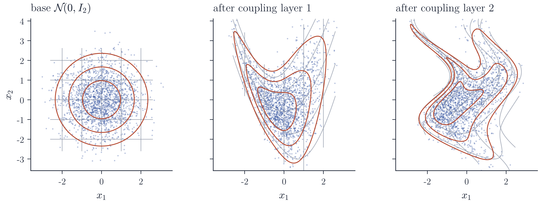
Figure 2 applies two hand-chosen layers in the plane: first $x_2 = u_2 e^{s_1(u_1)} + t_1(u_1)$ with $s_1(a) = 0.5\tanh a$ and $t_1(a) = 0.6a^2 - 0.6$, then $y_1 = x_1 e^{s_2(x_2)} + t_2(x_2)$ with $s_2(b) = -0.3\tanh b$ and $t_2(b) = 0.9\sin(1.2 b)$. The density contours are computed exactly by inverting the two layers:

import numpy as np
from scipy.stats import norm

def flow_logpdf(y1, y2, s1, t1, s2, t2):
    x1 = (y1 - t2(y2)) * np.exp(-s2(y2))   # undo layer 2
    u2 = (y2 - t1(x1)) * np.exp(-s1(x1))   # undo layer 1
    return norm.logpdf(x1) + norm.logpdf(u2) - s1(x1) - s2(y2)

Samples, deformed grid lines and density contours of a standard Gaussian before and after two affine coupling layers — Figure 2. Two affine coupling layers applied to $\mathcal N(0, I_2)$. Grey curves are the images of the segments $u_1 = c$ and $u_2 = c$, $c \in \{-2, -1, 0, 1, 2\}$, with the free coordinate in $[-2.6, 2.6]$; dots are $2000$ samples pushed through the layers; red curves are the contours at levels $0.01$, $0.04$ and $0.1$ of the exact density. The first layer moves points only vertically, the second only horizontally.

Autoregressive flows

An affine autoregressive flow lets every coordinate depend on all preceding ones. In the masked autoregressive flow (MAF) of Papamakarios, Pavlakou and Murray (2017),

\[x_i = \mu_i(x_{1:i-1}) + \exp\bigl(\alpha_i(x_{1:i-1})\bigr)\, u_i, \qquad i = 1, \dots, d,\]

with $\mu_1, \alpha_1$ constant. As a function of $u$ this map is lower triangular with $\partial x_i/\partial u_i = \exp(\alpha_i(x_{1:i-1}))$. Its inverse $u_i = (x_i - \mu_i(x_{1:i-1}))\exp(-\alpha_i(x_{1:i-1}))$ uses only observed coordinates, so given $x$ all $u_i$ are obtained in parallel by one pass of a network whose connections are masked to respect the ordering (the MADE construction of Germain, Gregor, Murray and Larochelle, 2015), and

\[\log p_X(x) = \sum_{i=1}^d \Bigl\{ \log\varphi(u_i) - \alpha_i(x_{1:i-1}) \Bigr\}.\]

Sampling, by contrast, is sequential: $x_i$ cannot be computed before $x_{1:i-1}$, which takes $d$ passes. The inverse autoregressive flow (IAF) of Kingma and coauthors (2016) conditions on $u_{1:i-1}$ instead, which reverses the trade-off: sampling, and evaluating the density of the flow’s own samples, takes one pass, while the density of an arbitrary point requires $d$ sequential steps. When $A$ consists of the first $k$ coordinates, a coupling layer is the special case in which $\mu_i$ and $\alpha_i$ depend only on the coordinates in $A$ and vanish for $i \in A$; it is cheap in both directions and less expressive per layer.

Maximum likelihood is a KL projection

Let $p_\theta$ be the density of $T_\theta(U)$ for a family of maps satisfying Theorem 1 with $\mathcal U = \mathcal X = \R^d$. Given observations $x_1, \dots, x_n$, the log-likelihood is computed from $\eqref{eq:composition}$, and its gradient in $\theta$ by automatic differentiation:

\[\ell_n(\theta) = \sum_{j=1}^n \Bigl\{ \log p_U\bigl(T_\theta^{-1}(x_j)\bigr) + \log\bigl\lvert \det J_{T_\theta^{-1}}(x_j)\bigr\rvert \Bigr\}.\]

Proposition 3. Let the data density $p^*$ satisfy $\int p^* \abs{\log p^*} < \infty$. Then for every $\theta$:

$\E_{p^*} \log p_\theta(X) = \E_{p^*} \log p^*(X) - \KL(p^* \,\Vert\, p_\theta)$, with both sides in $[-\infty, \infty)$;
$\KL(p^* \,\Vert\, p_\theta) = \KL(q^*_\theta \,\Vert\, p_U)$, where $q^*_\theta$ is the density of $T_\theta^{-1}(X)$ for $X \sim p^*$.

Proof. For part 1, write $\log p_\theta = \log p^* - \log(p^*/p_\theta)$ on $\{p^* > 0\}$. The negative part of $\log(p^*/p_\theta)$ is integrable under $p^*$, since $\log y \le y - 1$ gives $\int_{\{p^* < p_\theta\}} p^* \log(p_\theta/p^*) \le \int p_\theta \le 1$; hence $\KL(p^* \Vert p_\theta) = \E_{p^*}\log(p^*/p_\theta)$ is well defined in $[0, \infty]$, and the identity follows from linearity, using integrability of $\log p^*$. For part 2, Theorem 1 applied to $T_\theta^{-1}$ gives $q^*_\theta(u) = p^*(T_\theta(u))\,\lvert\det J_{T_\theta}(u)\rvert$, while $p_\theta(T_\theta(u)) = p_U(u) / \lvert \det J_{T_\theta}(u)\rvert$. The Jacobian factors cancel in the ratio:

\[\frac{q^*_\theta(u)}{p_U(u)} = \frac{p^*(T_\theta(u))}{p_\theta(T_\theta(u))} .\]

If $V \sim q^*_\theta$ then $T_\theta(V) \sim p^*$, so $\KL(q^*_\theta \Vert p_U) = \E \log\{q^*_\theta(V)/p_U(V)\} = \E_{p^*}\log\{p^*(X)/p_\theta(X)\}$.

Part 1 says that $\ell_n(\theta)/n$ is an unbiased estimate of $\E_{p^*}\log p_\theta(X)$, which differs from $-\KL(p^* \Vert p_\theta)$ by the constant $\E_{p^*}\log p^*(X)$, independent of $\theta$; maximum likelihood is the empirical version of projecting $p^*$ onto the model in forward Kullback–Leibler divergence. Part 2 explains the name. Fitting the flow is the same as choosing $T_\theta^{-1}$ so that the transformed data look like draws from the base distribution, so the inverse map normalizes the data, and a useful diagnostic for a fitted flow is to check the pulled-back sample $T_\theta^{-1}(x_j)$ against $\mathcal N(0, I_d)$.

The other direction of the divergence is used in variational inference, where the target $\pi = \tilde\pi/Z$ is known only up to its normalizing constant. Using $p_\theta(T_\theta(u)) = p_U(u)/\lvert\det J_{T_\theta}(u)\rvert$,

\[\KL(p_\theta \,\Vert\, \pi) = \E_{U \sim p_U}\Bigl[\log p_U(U) - \log\bigl\lvert \det J_{T_\theta}(U)\bigr\rvert - \log \tilde\pi\bigl(T_\theta(U)\bigr)\Bigr] + \log Z ,\]

which needs samples from the flow and the Jacobian at those samples, but no inverse. This is the setting of Rezende and Mohamed (2015) and the reason the IAF ordering suits variational inference. Because the expectation is over the fixed law of $U$, its gradient can be estimated by differentiating inside the expectation, which is justified when the derivative of the integrand in $\theta$ is dominated by an integrable function of $U$, uniformly for $\theta$ in a neighbourhood. The two directions behave differently: the forward divergence penalizes $p_\theta$ for missing mass of $p^*$, the reverse divergence penalizes $p_\theta$ for putting mass where $\pi$ has little.

Remarks

Theorem 1 also limits what a flow can represent. If $p_U > 0$ everywhere and $T$ is a diffeomorphism of $\R^d$, then $p_X > 0$ everywhere, so a target whose support is disconnected, or whose modes are separated by regions of near-zero density, can only be approximated, and approximating it well typically requires maps with very large Jacobian determinants or Lipschitz constants. A flow also preserves dimension. Data supported on a lower-dimensional set have no Lebesgue density, and for a sufficiently flexible family the likelihood is then unbounded; for discrete data such as images, which live on a lattice, this is avoided by adding uniform noise to the integer values before fitting (Theis, van den Oord and Bethge, A note on the evaluation of generative models, 2016). Continuous-time flows replace the composition by an ordinary differential equation $\dot z = f(z, t)$, along which $\tfrac{\dd}{\dd t}\log p(z(t)) = -\tr\, \partial f/\partial z$ (Chen, Rubanova, Bettencourt and Duvenaud, Neural ordinary differential equations, 2018); the trace replaces the determinant, and no triangular structure is needed.

The triangular construction of Proposition 2 goes back to Rosenblatt, Remarks on a multivariate transformation (Ann. Math. Statist., 1952), and Knothe, Contributions to the theory of convex bodies (Michigan Math. J., 1957). For the flows themselves, see Rezende and Mohamed, Variational inference with normalizing flows (ICML 2015), Dinh, Sohl-Dickstein and Bengio, Density estimation using Real NVP (ICLR 2017), Papamakarios, Pavlakou and Murray, Masked autoregressive flow for density estimation (NeurIPS 2017), and the review by Papamakarios, Nalisnick, Rezende, Mohamed and Lakshminarayanan, Normalizing flows for probabilistic modeling and inference (JMLR, 2021).