Objections to Bayesian inference, and the replies they have drawn

October 12, 2026Bayesian statistics

Bayesian inference has a short derivation and a long history of dispute. Given a model \(p(x \mid \theta)\) and a prior \(\pi(\theta)\), every inferential question is answered by the posterior \(\pi(\theta \mid x) \propto p(x \mid \theta)\pi(\theta)\), and decisions follow by minimizing posterior expected loss. Critics have never doubted the arithmetic. Their objections concern what the inputs mean, whether the outputs can be trusted, and whether the framework captures everything a scientist needs from statistics. Gelman (2008, Bayesian Analysis) collected many of these objections in a deliberately one-sided essay written in the voice of an imagined anti-Bayesian, and the published discussion and rejoinder answer it. The objections fall into six families. Each is stated below in its strongest form, followed by the main replies and by what seems to remain open.

1. The prior is subjective

The oldest objection is that the prior has no place in a scientific report. Fisher rejected inverse probability for most of his career on the grounds that a probability distribution for a fixed unknown constant has no frequency interpretation, and that two scientists with the same data but different priors would report different conclusions; his late book Statistical Methods and Scientific Inference gives his mature view. On this account a statistical method should let the data speak, and the prior is an uncontrolled ingredient that the reader cannot audit.

Three replies have been given, and they are not mutually consistent. The personalist reply, developed by de Finetti and by Savage in The Foundations of Statistics, accepts subjectivity and argues that it is unavoidable: an agent whose betting rates or preferences satisfy certain coherence axioms acts as if maximizing expected utility under some probability distribution, so the only question is whether that distribution is stated openly. The objective Bayesian reply, going back to Jeffreys’s Theory of Probability and continued in Bernardo’s reference priors (1979, Journal of the Royal Statistical Society, Series B), proposes rules that produce a prior from the model alone, so that different analysts using the same rule agree. The pragmatic reply, prominent in modern applied work, treats the prior as part of the model, on the same footing as the likelihood: both are assumptions, both can be motivated by substantive knowledge, and both can be checked against data.

The pragmatic reply has force against the strongest version of the objection, because the likelihood is rarely more objective than the prior. Choosing a normal error distribution, a linear predictor or an independence assumption is also a judgement, and it usually has a larger effect on conclusions than a weakly informative prior. What the reply concedes is that the prior’s influence must be reported and examined, for instance through sensitivity analysis. In small samples or weakly identified models that influence can be decisive.

2. Ignorance cannot be represented

If the prior is to be neutral, one wants a distribution expressing no information. The classical candidate, the uniform distribution, is not invariant under reparametrization. If \(\theta\) is a probability with a uniform prior on \((0, 1)\), the log-odds \(\eta = \log\{\theta/(1-\theta)\}\) has density

\[\pi_\eta(\eta) = \pi_\theta(\theta)\Bigl\lvert\frac{\dd\theta}{\dd\eta}\Bigr\rvert = \frac{e^\eta}{(1 + e^\eta)^2},\]

the standard logistic density, which is far from flat. Ignorance about \(\theta\) is knowledge about \(\eta\). This was one of Fisher’s arguments, and it shows that “no information” is not a property of a distribution alone; it depends on the parametrization in which it is expressed.

Jeffreys’s reply was to tie the prior to the model through the Fisher information, \(\pi(\theta) \propto \sqrt{I(\theta)}\). Under a smooth one-to-one reparametrization \(\eta = h(\theta)\), the information transforms as \(I_\eta(\eta) = I_\theta(\theta)\,(\dd\theta/\dd\eta)^2\), so

\[\sqrt{I_\eta(\eta)} = \sqrt{I_\theta(\theta)}\,\Bigl\lvert\frac{\dd\theta}{\dd\eta}\Bigr\rvert,\]

which is exactly the change-of-variables formula for densities. The rule therefore gives the same prior whichever parametrization is used; for a Bernoulli probability it gives \(\mathrm{Beta}(\tfrac12, \tfrac12)\). The reply is successful in one dimension and less so beyond it. Jeffreys himself modified the rule for location–scale problems, the multiparameter version can give poor answers, and reference priors depend on an ordering of parameters by importance. Improper default priors also generate their own difficulties, including the marginalization paradoxes of Dawid, Stone and Zidek (1973, Journal of the Royal Statistical Society, Series B) and posteriors that fail to exist. Kass and Wasserman (1996, Journal of the American Statistical Association) surveyed the formal rules and concluded, roughly, that each is useful as a convention but none has a claim to represent ignorance. Most contemporary Bayesians accept this and use priors that are deliberately but weakly informative.

3. Frequentist performance is not guaranteed

A frequentist critic can grant the Bayesian everything about interpretation and still ask how the procedure behaves under repeated sampling from a fixed truth. A 95% credible interval need not cover the true parameter 95% of the time, and posterior consistency, the requirement that the posterior concentrate at the truth as data accumulate, is not automatic. Freedman (1963) and Diaconis and Freedman (1986, Annals of Statistics) gave examples of natural nonparametric priors whose posteriors converge to the wrong answer. In semiparametric problems the difficulty is sharper. Robins and Ritov (1997, Statistics in Medicine) described a missing-data problem in which the probability of observing each unit is known by design, a simple weighted estimator is consistent at the usual rate, and yet a Bayesian analysis whose likelihood does not involve those known probabilities cannot achieve that rate uniformly over a large model. Wasserman and others have used this example to argue that likelihood-based inference can be the wrong tool when the design carries information that the likelihood ignores.

The replies come in two kinds. For regular parametric models the Bernstein–von Mises theorem shows that the posterior is asymptotically normal, centred at an efficient estimator with the inverse Fisher information as covariance, so credible sets are asymptotically confidence sets; much of the disagreement disappears in large samples. For nonparametric problems, a substantial theory now gives conditions on the prior under which posteriors are consistent and contract at optimal rates (see Ghosal and van der Vaart, Fundamentals of Nonparametric Bayesian Inference), and its existence is a concession that frequentist properties matter to Bayesians too. In the Robins–Ritov example, Bayesians have proposed priors that depend on the known design probabilities, which restores good behaviour at the cost of a prior that is hard to justify on purely subjective grounds. Little (2006, The American Statistician) describes the resulting position as calibrated Bayes: inference is carried out by Bayes’ theorem, and models and priors are chosen and checked partly for their frequentist calibration.

4. The likelihood principle and stopping rules

Bayesian inference depends on the data only through the likelihood function. This implies the likelihood principle: two experiments that produce proportional likelihoods for \(\theta\) must lead to the same inference. Birnbaum (1962, Journal of the American Statistical Association) argued that the principle follows from two weaker principles, sufficiency and conditionality, that most frequentists accept; Mayo (2014, Statistical Science) disputes the validity of that derivation, and the debate continues. Frequentist procedures violate the principle routinely, because p-values and confidence levels depend on the sampling distribution of the data, and therefore on outcomes that could have occurred but did not.

A standard example shows the conflict. Twelve independent Bernoulli(\(\theta\)) trials produce three successes and nine failures, and we test \(\theta = \tfrac12\) against \(\theta < \tfrac12\). If the number of trials was fixed at 12, the number of successes \(X\) is binomial and the p-value is

\[\P_{1/2}(X \le 3) = \frac{1 + 12 + 66 + 220}{2^{12}} = \frac{299}{4096} \approx 0.073 .\]

If instead the experimenter sampled until the third success, which happened on trial 12, the number of trials \(N\) is negative binomial, and small values of \(\theta\) make large \(N\) likely, so the p-value is

\[\P_{1/2}(N \ge 12) = \P_{1/2}(\text{at most two successes in 11 trials}) = \frac{1 + 11 + 55}{2^{11}} = \frac{67}{2048} \approx 0.033 .\]

The two designs disagree at the 5% level. Both likelihoods are proportional to \(\theta^3(1-\theta)^9\), so any Bayesian analysis with a given prior reaches the same conclusion under both; with a uniform prior the posterior is \(\mathrm{Beta}(4, 10)\) and \(\P(\theta \ge \tfrac12 \mid \text{data}) \approx 0.046\) (Figure 1).

Figure 1. Three successes in twelve Bernoulli trials. Left: null distribution of the number of successes when $n = 12$ is fixed; the shaded tail gives $p = 0.073$. Middle: null distribution of the trial $N$ on which the third success occurs; the shaded tail gives $p = 0.033$. Right: the likelihood $\theta^3(1-\theta)^9$ is the same in both designs, and so is the posterior under a uniform prior, $\mathrm{Beta}(4, 10)$, with $P(\theta \ge 1/2 \mid \text{data}) = 0.046$.

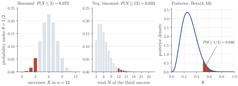
Whether this is a strength or a defect is the substance of the dispute. Bayesians regard the irrelevance of the stopping rule as a merit: the experimenter’s intentions about what would have happened in other circumstances should not change what the observed data say. Critics, including Mayo in Statistical Inference as Severe Testing (2018), regard it as a defect, because it allows optional stopping. The sharpest version, pressed by Armitage in the 1960s, concerns sampling until a desired conclusion is reached. Let \(X_1, X_2, \dots\) be independent \(N(\theta, 1)\), and let the prior on \(\theta\) be flat, so that the 95% credible interval after \(n\) observations is \(\bar X_n \pm 1.96/\sqrt n\). If \(\theta = 0\), the interval excludes zero exactly when \(\abs{S_n} > 1.96\sqrt n\), where \(S_n = X_1 + \dots + X_n\). By the law of the iterated logarithm, \(\limsup_n \abs{S_n}/\sqrt{2n\log\log n} = 1\) almost surely, so this happens for infinitely many \(n\) with probability one. An experimenter who stops as soon as the interval excludes zero will therefore, with certainty, eventually report a credible interval that excludes the true value.

Two replies are available. The first is that the example uses an improper prior that gives no weight to the possibility \(\theta = 0\) exactly; with a proper prior that gives positive probability to \(\theta = 0\), the relevant quantity is the Bayes factor, and Bayes factors resist optional stopping in a precise sense.

Proposition 1. Let \(X_1, X_2, \dots\) be independent with density \(f_0 > 0\) under \(H_0\), and let \(m_n(x_1, \dots, x_n) = \int \prod_{i \le n} f_\theta(x_i)\,\Pi(\dd\theta)\) be the marginal density under \(H_1\) for a proper prior \(\Pi\). Then \(B_n = m_n(X_1, \dots, X_n)/\prod_{i \le n} f_0(X_i)\) is a nonnegative martingale under \(H_0\) with \(\E_0 B_n = 1\), and for every \(k > 1\)

\[\P_0\bigl(B_n \ge k \text{ for some } n\bigr) \le \frac1k .\]

Proof. Conditionally on \(X_1, \dots, X_n\), the ratio \(m_{n+1}(X_1, \dots, X_n, x)/m_n(X_1, \dots, X_n)\) is the predictive density of the next observation under \(H_1\) (where \(m_n > 0\)), so

\[\E_0[B_{n+1} \mid X_1, \dots, X_n] = B_n \int \frac{m_{n+1}(X_1, \dots, X_n, x)}{m_n(X_1, \dots, X_n)\, f_0(x)} f_0(x)\,\dd x = B_n ,\]

and on \(\{m_n = 0\}\) both sides vanish. Hence \(\E_0 B_n = \E_0 B_1 = 1\). The inequality is Ville’s maximal inequality for nonnegative supermartingales: with \(\tau = \inf\{n : B_n \ge k\}\), optional stopping at the bounded time \(\tau \wedge N\) gives \(k\,\P_0(\tau \le N) \le \E_0 B_{\tau \wedge N} \le 1\), and one lets \(N \to \infty\).

An experimenter who samples until the Bayes factor against a true simple null reaches 20 succeeds with probability at most 5%, however long the sampling continues. The second reply concedes the critic’s point for interval estimation and answers that a posterior interval is a statement of belief given the data, which optional stopping does not invalidate if the prior is honest. That reply does not satisfy a critic whose concern is the reliability of the procedure, and here the two sides are answering different questions.

5. The model is never questioned

A posterior distribution is conditional on the model. Bayes’ theorem redistributes probability among the parameter values the model allows, and has nothing to say if the model is wrong. Box (1980, Journal of the Royal Statistical Society, Series A) argued that statistical work alternates between criticism and estimation, that estimation is naturally Bayesian, and that criticism requires comparing the data with what the model predicts, a sampling-theory activity that the formal Bayesian calculus does not include. Strict subjectivists have difficulty with this, because checking a model against the data that also fitted it uses the data twice.

Modern practice largely follows Box. Posterior predictive checks (Gelman, Meng and Stern, 1996, Statistica Sinica) compare observed data with replications drawn from the fitted model, and cross-validation is used routinely to compare models. Gelman and Shalizi (2013, British Journal of Mathematical and Statistical Psychology) argue that this practice is better described as hypothetico-deductive than as inductive updating of belief: models are proposed, used to derive consequences and rejected when the consequences fail, with Bayesian inference serving as the engine within a model. On this view the objection is correct about the formal theory and mistaken about how Bayesian statistics is done. A subjectivist can reply that the larger model, including alternatives, should have been in the prior from the start; the practical difficulty is that nobody can write down all the alternatives in advance.

6. Hypothesis tests are fragile

Bayes factors for nested hypotheses depend strongly on the prior under the alternative, even in large samples. For a point null on a normal mean with a \(N(\theta_0, \tau^2)\) prior under the alternative, the Bayes factor at fixed \(z\)-statistic grows like \(\tau\sqrt n\), so the same data that reject the null at the 1% level can favour it heavily (Lindley’s paradox), and a vague alternative prior favours the null without limit. Improper priors cannot be used at all, since their arbitrary constants enter the Bayes factor. Critics take this as evidence that Bayesian testing rests on arbitrary choices. Defenders reply that the sensitivity is real and informative, because a point null and a diffuse alternative are different scientific claims, and that the p-value’s apparent stability hides the fact that it answers a different question. Many Bayesians avoid the issue by preferring estimation of effect sizes to testing, or by using default Bayes factors whose alternative priors are scaled to the information in a single observation. Neither move is accepted by everyone.

Computation, then and now

For much of the twentieth century a further objection was simply that posteriors could not be computed outside conjugate models. Markov chain Monte Carlo, brought into mainstream statistics around 1990 by Gelfand and Smith (1990, Journal of the American Statistical Association) among others, removed it as an objection of principle. A residual version survives. Samplers can fail silently on multimodal or poorly identified posteriors, and fast approximations such as variational inference produce distributions that are not posteriors and whose errors are hard to assess. These are concerns about the reliability of numerical approximations, and the remedies, diagnostics, simulation-based calibration and careful parametrization, are technical; they do not distinguish Bayesian from other computationally heavy methods.

Where matters stand

Several of the classical objections have changed character. The demand for an objective prior has largely been abandoned on both sides; few frequentists now claim that their own modelling choices are free of judgement, and few Bayesians claim that a default prior represents ignorance. The frequentist evaluation of Bayesian procedures has become a branch of Bayesian theory. The disagreements that remain are about the likelihood principle, about testing, and about whether statistical evidence should measure the reliability of a procedure or the support for a hypothesis given the data. These are questions about the purpose of inference, and the calculus of probability alone does not settle them. Efron’s essay “Why isn’t everyone a Bayesian?” (1986, The American Statistician) and Gelman’s 2008 essay, each with its published discussion, are good entry points to the debate in the critics’ and defenders’ own terms.